Content from Python Fundamentals

---

Last updated on 2026-03-30 | Edit this page

Estimated time: 30 minutes

Overview

Questions

• How do we process mathematical operations in Python?
• What happens if we make a mistake?

Objectives

• Become familiar with mathematical operators and built-in functions.
• Become more confident using Jupyter notebooks (e.g., writing and running cells).
• Understand the order of operations.

Simple calculation

---

Any Python interpreter can be used as a calculator:

Subtraction

PYTHON

10 - 5 #(subtraction) 

OUTPUT

5

Addition

PYTHON

10 + 5 #(addition) 

OUTPUT

15

Multiplication

PYTHON

10 * 5 #(multiplication) 

OUTPUT

50

Division

PYTHON

10 / 5 #(division) 

OUTPUT

2.0

Exponentiation

PYTHON

5 ** 2 #(exponentiation) 

OUTPUT

25

Modulus

PYTHON

10 % 3 #(modulus)  

OUTPUT

1

Note: anything following a ‘#’ is considered a comment. Comments are not read by Python, they are used to help explain the code to other users (and your future self).

Order of operations

Question: Before you enter the next calculation, take a second to consider what answer you would expect.

PYTHON

6 + 9 / 3 

OUTPUT

9.0

If the answer was not what you were expecting you will need to become clear on order of operations in Python.

Remember BO(DM)(AS) (BIDMAS or PEMDAS)

• Brackets

• Orders

• Division/Multiplication*

• Addition/Subtraction*

Operators with the same precedence are calculated left to right.

This tells you the order in which mathematical operations will be performed and ensures consistency during evaluation.

To make this concept clearer, try:

PYTHON

(6 + 9) / 3 

OUTPUT

5.0

Using brackets we have manipulated the order of operations to perform the addition before the division. Be conscious of how you structure your mathematical operations to ensure the desired results but also readability of your code.

So what happens if we do something wrong? I am worried that I might break something!

If we do something wrong, Python will usually show us an error message. Sometimes, more frustratingly, the code will still run but produce unexpected results. This is a normal part of programming and not usually a sign that you have broken anything. So, how do we get help when things don’t work like they should?

Getting Help

---

We are now going to briefly explore how to find help in Python and introduce our first built-in function. The built-in function we will use is help(), which displays information about Python objects. We will use it to look up another built-in function, print().

Callout

A function is a named piece of code that performs a task. We will look at functions in more detail later in the module. For now, we will use built-in functions (functions included in base Python) to understand how to use them.

Every built-in function has extensive documentation that can also be found online.

PYTHON

help(print)

OUTPUT

Help on built-in function print in module builtins:

print(*args, sep=' ', end='\n', file=None, flush=False)
    Prints the values to a stream, or to sys.stdout by default.

    sep
      string inserted between values, default a space.
    end
      string appended after the last value, default a newline.
    file
      a file-like object (stream); defaults to the current sys.stdout.
    flush
      whether to forcibly flush the stream.

This help message (the function’s “docstring”) includes a usage statement, a list of parameters accepted by the function, and their default values if they have them.

It is normal to encounter error messages while programming, whether you are learning for the first time or have been programming for many years. We will discuss error messages in more detail later. For now, let’s explore how people use them to get more help when they are stuck with their Python code.

• Search the internet: paste the last line of your error message or the word “python” and a short description of what you want to do into your favourite search engine and you will usually find several examples where other people have encountered the same problem and came looking for help.
  • Stack Overflow can be particularly helpful for this: answers to questions are presented as a ranked thread ordered according to how useful other users found them to be.
  • Take care: copying and pasting code written by somebody else is risky unless you understand exactly what it is doing!
• Ask somebody “in the real world”. If you have a colleague or friend with more expertise in Python than you have, show them the problem you are having and ask them for help.

We will discuss more debugging strategies in greater depth later in the lesson.

Key Points

• Built-in functions are always available to use (without additional libraries).
• Use help(thing) to view help for something.
• You may have seen some error messages already, they provide information about what has gone wrong with your code and where.

Content from Variables and basic data types

---

Last updated on 2026-03-30 | Edit this page

Estimated time: 45 minutes

Overview

Questions

• What is a variable?
• What is a type?
• Why are types important?
• What happens when notebook cells are run out of order?

Objectives

• Understand the syntax behind assigning values to variables in Python.
• Recognise common Python data types and understand why they matter.
• Understand that Jupyter notebooks run cells in the order you execute them, not the order they appear.

Variables

---

To do anything useful with data, we need to assign its value to a variable. In Python, we can assign a value to a variable, using the equals sign =. For example, we can track the weight of a patient who weighs 60 kilograms by assigning the value 60 to a variable weight_kg:

Callout

In Python, = means assignment. It tells Python to store a value in a variable, it does not ask whether two things are equal. Later we will encounter == this is a check for equivalence.

PYTHON

weight_kg = 60

From now on, whenever we use weight_kg, Python will substitute the value we assigned to it. In simple terms, a variable is a name for a value.

In Python, variable naming has rules:

• Variable names are case-sensitive (My_name is different from my_name).

• They can not contain spaces (e.g. my name =)

• They must start with a letter or an underscore.

• They can consist of letters, numbers, and underscores.

• Some reserved words (e.g., 'else', 'for') cannot be used as variable names because they already have a specific meaning in Python.

This means that, for example:

• weight0 is a valid variable name, whereas 0weight is not
• weight and Weight are different variables

It may seem there are many restrictions but there are actually a huge number of variable naming combinations. However, just because you can use weird and wonderful combinations, doesn’t mean you should. There are several naming conventions in the Python community that help provide structure and consistency.

1. my_variable (underscore or snake case)

2. myVariable (camel case)

Although some may violently disagree with us, we believe for most coders it does not matter which convention you pick. In Python, snake_case is the most common naming convention for variables, so it is a good default choice for beginners. More importantly, there are two key principles for variable naming that will make your life easier:

1. Consistency - pick a convention and stick with it.

2. Succinctness - Keep variable names short, readable, and descriptive.

For example, if you wanted a variable name for a temperature reading taken in Aberystwyth:

This:

min_temp_aber_C

Is better than this:

temp

Or this:

theminimumtemperaturerecordedfromaberystwythindegreescelsius

Being consistent, aware of context, and conscious of your variable naming will make reading your code easier and decrease the risk of errors.

Callout

WARNING: The first of many unfunny computer science jokes.

“There are only two hard problems in Computer Science: cache invalidation and naming things.” – Phil Karlton

Types of data

---

Python utilises different data types to efficiently store and manipulate different kinds of data. A type tells Python what kind of value something is, such as a whole number, a decimal number, or text. Python is dynamically typed, this means that you do not need to specify a data type when you declare a variable. You provide the variable name and the value you want to store, and Python handles the data type automatically. We will look at the most common data types in Python.

Data Type	Description	Example
int	Integer data type	42
float	Floating-point data type	3.14
str	String data type	‘hello’
bool	Boolean data type	True, False
NoneType	NoneType data type (represents null value)	None

In the example above, variable weight_kg has an integer value of 60. If we want to more precisely track the weight of our patient, we can use a floating point value by executing:

PYTHON

weight_kg = 60.3

To create a string, we add single or double quotes around some text. To identify and track a patient throughout our study, we can assign each person a unique identifier by storing it in a string:

PYTHON

patient_id = '001'

Built-in Python functions

---

To carry out common tasks with data and variables in Python, the language provides us with several built-in functions. To display information to the screen, we use the print() function:

PYTHON

print(weight_lb)
print(patient_id)

OUTPUT

132.66
inflam_001

When we want to make use of a function, referred to as calling the function, we follow its name by parentheses. The parentheses are important: if you leave them off, the function doesn’t actually run! Sometimes you will include values or variables inside the parentheses for the function to use. In the case of print(), we use the parentheses to tell the function what value we want to display. We will learn more about how functions work and how to create our own in later episodes.

We can display multiple things at once using only one print() call:

PYTHON

print(patient_id, 'weight in kilograms:', weight_kg)

OUTPUT

inflam_001 weight in kilograms: 60.3

We can also call a function inside another function call. For example, Python has a built-in function called type() that tells you a value’s data type:

PYTHON

print(type(60.3))
print(type(patient_id))

OUTPUT

<class 'float'>
<class 'str'>

Moreover, we can do arithmetic with variables right inside the print() function:

PYTHON

print('weight in pounds:', 2.2 * weight_kg)

OUTPUT

weight in pounds: 132.66

The above command, however, did not change the value of weight_kg:

PYTHON

print(weight_kg)

OUTPUT

60.3

To change the value of the weight_kg variable, we have to assign weight_kg a new value using the equals = sign:

PYTHON

weight_kg = 65.0
print('weight in kilograms is now:', weight_kg)

OUTPUT

weight in kilograms is now: 65.0

Using Variables in Python

---

Once we have data stored with variable names, we can make use of it in calculations. We may want to store our patient’s weight in pounds as well as kilograms:

PYTHON

weight_lb = 2.2 * weight_kg

We might decide to add a prefix to our patient identifier:

PYTHON

patient_id = 'inflam_' + patient_id

How Python Assigns Data Types

---

Dynamic Typing

In Python, you don’t declare a variable’s type explicitly. Instead, the type is determined automatically when you assign a value.

PYTHON

x = 10        # x is an int
print(x)
x = "hello"   # now x is a string
print(x)

PYTHON

10
hello

For example, depending on how you assign a value, Python automatically determines its type:

PYTHON

a = 5
b = 5.0
c = "5"

print(type(a))  # int
print(type(b))  # float
print(type(c))  # str

PYTHON

<class 'int'>
<class 'float'>
<class 'str'>

Different data types behave differently. Some can be combined directly, such as integers and floats, but others cannot. For example, strings cannot be added to numbers in a meaningful way without conversion.

Another challenge with dynamic typing is that sometimes values that look like numbers are actually stored as strings. This can lead to unexpected behaviour, as shown below:

PYTHON

x = "10"        

To use this value as a number, we need to convert it from a string to an integer:

PYTHON

print(type(x))       
x = int(x)
print(type(x))

PYTHON

<class 'str'>
<class 'int'>

Running code in order

---

Jupyter notebooks keep variables, imports, and results in memory as you run cells. That means each cell can depend on work done earlier. When cells are run out of order, the notebook can end up in a state where the code looks fine but behaves unpredictably.

Running cells in order makes the notebook:

• easier to understand
• easier to debug
• easier for other people to reproduce
• less likely to break because of hidden state

A notebook is not just a document. It is also a live coding session.

If, during your work, you add something in cell 8 that cell 3 depends on, your notebook may still appear to work because both cells have already been run in your current session. However, if someone opens the notebook from scratch and runs the cells in order, they may get an error.

Examples

PYTHON

# Cell 1
x = 10

PYTHON

# Cell 2
y = x + 5
print(y)

If Cell 2 is run before Cell 1, Python will raise an error because x does not exist yet.

Problems caused by running out of order

• Name errors: variables or functions are missing
• Old values: variables keep outdated data from earlier runs
• Confusing bugs: results change for no obvious reason
• Poor reproducibility: others cannot get the same output
• Hidden dependencies: a cell works only because of some earlier unseen action

Challenge

Check Your Understanding

What values do the variables mass and age have after each of the following statements? Test your answer by executing the lines.

PYTHON

mass = 47.5 #1
age = 122 #2
mass = mass * 2.0 #3
age = age - 20 #4

Show me the solution

OUTPUT

at 1 `mass` holds a value of 47.5, `age` does not exist
at 2 `mass` still holds a value of 47.5, `age` holds a value of 122
at 3 `mass` now has a value of 95.0, `age`'s value is still 122
at 4 `mass` still has a value of 95.0, `age` now holds 102

Key Points

• Basic data types in Python include integers, strings, and floating-point numbers.
• Use variable = value to assign a value to a variable in order to record it in memory.
• Variables are created on demand whenever a value is assigned to them.
• Use print(something) to display the value of something.
• Use # some kind of explanation to add comments to programs.

Content from Lists and dictionaries

---

Last updated on 2026-03-30 | Edit this page

Estimated time: 60 minutes

Overview

Questions

• What is the difference between a list and a dictionary?
• Why do we use a list or dictionary instead of lots of separate variables?
• When is one data structure a better choice than another?
• How do I get a value out of a data structure?
• Can I get multiple values out of a data structure?

Objectives

• Understand why data structures are useful for storing multiple values.
• Create, inspect, index, and modify data structures in Python.
• Understand the difference between mutable and immutable objects.
• Understand that data structures can be nested to suit our storage needs.

Python lists

---

We create a list by putting values inside square brackets and separating the values with commas:

PYTHON

odds = [1, 3, 5, 7]
print('odds are:', odds)

OUTPUT

odds are: [1, 3, 5, 7]

We can access elements of a list using indices – numbered positions of elements in the list. These positions are numbered starting at 0, so the first element has an index of 0.

PYTHON

print('first element:', odds[0])
print('last element:', odds[3])
print('"-1" element:', odds[-1])

OUTPUT

first element: 1
last element: 7
"-1" element: 7

Yes, we can use negative numbers as indices in Python. When we do so, the index -1 gives us the last element in the list, -2 the second to last, and so on. Because of this, odds[3] and odds[-1] point to the same element here.

There is one important difference between lists and strings: we can change the values in a list, but we cannot change individual characters in a string. For example:

PYTHON

names = ['Curie', 'Darwing', 'Turing']  # typo in Darwin's name
print('names is originally:', names)
names[1] = 'Darwin'  # correct the name
print('final value of names:', names)

OUTPUT

names is originally: ['Curie', 'Darwing', 'Turing']
final value of names: ['Curie', 'Darwin', 'Turing']

Callout

Ch-Ch-Ch-Ch-Changes

Mutable data (like lists and arrays) can be changed after creation, while immutable data (like strings and numbers) cannot be modified, only replaced. Modifying mutable objects in place can lead to unexpected behaviour if multiple variables reference the same data. To avoid this, you can create a copy so changes do not affect the original. In-place changes are more efficient but can make code harder to understand, so there is a trade-off between clarity and performance.

PYTHON

mild_salsa = ['peppers', 'onions', 'cilantro']
hot_salsa = mild_salsa        # <-- mild_salsa and hot_salsa point to the *same* list data in memory
hot_salsa[0] = 'hot peppers'
print('Ingredients in mild salsa:', mild_salsa)
print('Ingredients in hot salsa:', hot_salsa)

OUTPUT

Ingredients in mild salsa: ['hot peppers', 'onions', 'cilantro']
Ingredients in hot salsa: ['hot peppers', 'onions', 'cilantro']

If you want variables with mutable values to be independent, you must make a copy of the value when you assign it.

PYTHON

mild_salsa = ['peppers', 'onions', 'cilantro']
hot_salsa = mild_salsa.copy()        # <-- hot_salsa is now a copy of the original
hot_salsa[0] = 'hot peppers'
print('Ingredients in mild salsa:', mild_salsa)
print('Ingredients in hot salsa:', hot_salsa)

OUTPUT

Ingredients in mild salsa: ['peppers', 'onions', 'cilantro']
Ingredients in hot salsa: ['hot peppers','onions', 'cilantro']

Callout

Nested Lists

Since a list can contain any Python variables, it can even contain other lists.

For example, you could represent the products on the shelves of a small grocery shop as a nested list called veg:

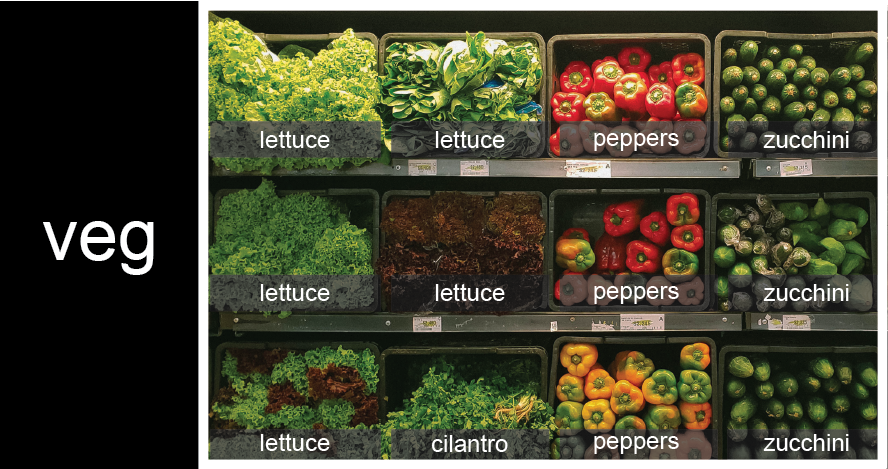
To store the contents of the shelf in a nested list, you write it this way:

PYTHON

veg = [['lettuce', 'lettuce', 'peppers', 'zucchini'],
     ['lettuce', 'lettuce', 'peppers', 'zucchini'],
     ['lettuce', 'cilantro', 'peppers', 'zucchini']]

Here are some visual examples of how indexing a list of lists veg works. First, you can reference each row on the shelf as a separate list. For example, veg[2] represents the bottom row, which is a list of the baskets in that row.

Index operations using the image would work like this:

PYTHON

print(veg[2])

OUTPUT

['lettuce', 'cilantro', 'peppers', 'zucchini']

PYTHON

print(veg[0])

OUTPUT

['lettuce', 'lettuce', 'peppers', 'zucchini']

To reference a specific basket on a specific shelf, you use two indexes. The first index represents the row (from top to bottom) and the second index represents the specific basket (from left to right).

PYTHON

print(veg[0][0])

OUTPUT

'lettuce'

PYTHON

print(veg[1][2])

OUTPUT

'peppers'

Callout

Heterogeneous Lists

Lists in Python can contain elements of different types. Example:

PYTHON

sample_ages = [10, 12.5, 'Unknown']

There are many ways to change the contents of lists besides assigning new values to individual elements:

Adding to list

To append an item to a list

PYTHON

odds.append(11)
print('odds after adding a value:', odds)

Removing elements

PYTHON

removed_element = odds.pop(0)
print('odds after removing the first element:', odds)
print('removed_element:', removed_element)

List slicing

If you want to take a slice from the beginning of a sequence, you can omit the first index in the range:

PYTHON

date = 'Monday 4 January 2016'
day = date[0:6]
print('Using 0 to begin range:', day)
day = date[:6]
print('Omitting beginning index:', day)

OUTPUT

Using 0 to begin range: Monday
Omitting beginning index: Monday

And similarly, you can omit the ending index in the range to take a slice to the very end of the sequence:

PYTHON

months = ['jan', 'feb', 'mar', 'apr', 'may', 'jun', 'jul', 'aug', 'sep', 'oct', 'nov', 'dec']
sond = months[8:12]
print('With known last position:', sond)
sond = months[8:len(months)]
print('Using len() to get last entry:', sond)
sond = months[8:]
print('Omitting ending index:', sond)

OUTPUT

With known last position: ['sep', 'oct', 'nov', 'dec']
Using len() to get last entry: ['sep', 'oct', 'nov', 'dec']
Omitting ending index: ['sep', 'oct', 'nov', 'dec']

Challenge

Slicing From the End

Use slicing to access only the last four characters of a string or entries of a list.

PYTHON

string_for_slicing = 'Observation date: 02-Feb-2013'
list_for_slicing = [['fluorine', 'F'],
                    ['chlorine', 'Cl'],
                    ['bromine', 'Br'],
                    ['iodine', 'I'],
                    ['astatine', 'At']]

OUTPUT

'2013'
[['chlorine', 'Cl'], ['bromine', 'Br'], ['iodine', 'I'], ['astatine', 'At']]

Would your solution work regardless of whether you knew beforehand the length of the string or list (e.g. if you wanted to apply the solution to a set of lists of different lengths)? If not, try to change your approach to make it more robust.

Hint: Remember that indices can be negative as well as positive

Show me the solution

Use negative indices to count elements from the end of a container (such as list or string):

PYTHON

string_for_slicing[-4:]
list_for_slicing[-4:]

Challenge

Non-Continuous Slices

So far we’ve seen how to use slicing to take single blocks of successive entries from a sequence. But what if we want to take a subset of entries that aren’t next to each other in the sequence?

You can achieve this by providing a third argument to the range within the brackets, called the step size. The example below shows how you can take every third entry in a list:

PYTHON

primes = [2, 3, 5, 7, 11, 13, 17, 19, 23, 29, 31, 37]
subset = primes[0:12:3]
print('subset', subset)

OUTPUT

subset [2, 7, 17, 29]

Notice that the slice taken begins with the first entry in the range, followed by entries taken at equally-spaced intervals (the steps) thereafter. If you wanted to begin the subset with the third entry, you would need to specify that as the starting point of the sliced range:

PYTHON

primes = [2, 3, 5, 7, 11, 13, 17, 19, 23, 29, 31, 37]
subset = primes[2:12:3]
print('subset', subset)

OUTPUT

subset [5, 13, 23, 37]

Use the step size argument to create a new string that contains only every other character in the string “In an octopus’s garden in the shade”. Start with creating a variable to hold the string:

PYTHON

beatles = "In an octopus's garden in the shade"

What slice of beatles will produce the following output (i.e., the first character, third character, and every other character through the end of the string)?

OUTPUT

I notpssgre ntesae

Show me the solution

To obtain every other character you need to provide a slice with the step size of 2:

PYTHON

beatles[0:35:2]

You can also leave out the beginning and end of the slice to take the whole string and provide only the step argument to go every second element:

PYTHON

beatles[::2]

Dictionaries

---

• Dictionaries store key-value pairs and are accessed using keys rather than numeric positions.
• They are mutable, and keys are often strings or numbers.
• Dictionaries are created using curly braces {}.

Example of dictionary creation:

PYTHON

my_dict = {'name': 'John', 'age': 30, 'city': 'New York'}

Accessing elements:

• Elements in a dictionary are accessed using square brackets [] and keys.

Example of accessing elements:

PYTHON

person_name = my_dict['name']   # Accessing value corresponding to 'name' key

Manipulating dictionaries:

• Dictionaries support various operations like adding, removing, and updating key-value pairs.

Examples of manipulation:

PYTHON

my_dict['gender'] = 'Male'     # Adds 'gender': 'Male' to the dictionary
del my_dict['age']             # Removes the key 'age' and its value
my_dict['city'] = 'Los Angeles' # Updates the value of 'city' key to 'Los Angeles'

Why do we need different data structures?

---

We need different data structures because data does not always come in the same form.

Sometimes we want to store values in a simple ordered collection. A list is good for this. For example, a list works well for a sequence of numbers, names, or measurements where the position of each item matters.

Sometimes we want to store values with labels. A dictionary is good for this. For example, if we want to store a person’s name, age, and job, it is more useful to label each value than to rely on its position.

So, lists and dictionaries are both ways of storing multiple values, but they are designed for different purposes. A list helps us work with order, while a dictionary helps us work with meaningful labels.

We also need to consider how information is accessed when working with data at scale, particularly when thinking about how efficiently we can search for values within different data structures.

Key Points

• [value1, value2, value3, ...] creates a list, (this process does not have to be manual).
• Lists can contain any Python object, including lists (i.e., list of lists).
• Lists are indexed and sliced with square brackets (e.g., list[0] and list[2:9]), in the same way as strings and arrays.
• Dictionaries are indexed with the key (e.g., dictionary[‘first_entry’])
• Some objects are mutable (e.g., lists).
• Some objects are immutable (e.g., strings).
• Different data structures exist because they support different ways of organising and accessing information.

Content from Libraries and imports

---

Last updated on 2026-03-30 | Edit this page

Estimated time: 30 minutes

Overview

Questions

• Why do we need libraries?
• What does import ... as ... do?

Objectives

• Install and import libraries.
• Understand how libraries relate to environments.

What is a library?

---

A library is a collection of ready-made code written by other programmers that you can use in your own program.

Instead of building every tool yourself, you can borrow tools that already exist. A library might contain code for:

• doing calculations
• working with data
• drawing graphs
• making games
• handling dates and times

You can think of a library like a toolbox. If you need a hammer, you do not make one from metal and wood first, you take one from the toolbox and use it. In programming, a library is that toolbox.

Why do programmers use libraries?

---

Programmers use libraries because they save time and effort.

If somebody has already written code that works well, it makes sense to use it rather than create the same thing again. Libraries help us:

• work faster
• avoid repeating work
• use tested and reliable code
• solve bigger problems more easily

This is one reason programming is powerful: we build on work that already exists.

Why do we not write everything from scratch?

---

Writing everything from scratch would take far too long and would often lead to more mistakes.

Imagine you wanted to create a graph, analyse a large dataset, or generate random numbers. You could try to write all that code yourself, but it would be slow, difficult, and unnecessary.

Instead, we use libraries because:

• they are already written
• they are usually tested by many people
• they let us focus on solving the actual problem
• they make programs shorter and clearer

So rather than spending hours rebuilding common tools, we use libraries and spend our time on the parts that are unique to our project.

What does import mean?

---

To use a library in Python, we usually import it.

Callout

If you have never used Python before, or if you are not using the Carpentries environment, you may need to install some packages first.

PYTHON

%pip install [PACKAGE NAME]

The word import tells Python to load the library so we can use its tools in our code.

For example:

PYTHON

import math

This imports the math library, which contains useful mathematical functions.

After that, we can use parts of the library like this:

PYTHON

print(math.sqrt(16))

This prints the square root of 16.

What does import … as … mean?

---

Sometimes library names are long, or programmers want a shorter name to type. Python lets us rename a library when we import it.

For example:

PYTHON

import numpy as np

This imports the library numpy but gives it the shorter name np inside our code.

Now instead of writing:

PYTHON

numpy.array([1, 2, 3])

we write:

PYTHON

np.array([1, 2, 3])

This is quicker and easier to read once you know the shortcut.

Why use import … as …?

We use import … as … because:

• it saves typing
• it makes code neater
• short names are often standard and widely recognised

For example:

• numpy as np
• pandas as pd
• matplotlib.pyplot as plt

These short versions are commonly used, so using them can make code easier for others to recognise.

Packages, versions, and environments

---

Packages are updated over time, so different versions of the same package can behave differently.

In simple projects this may not matter much, but larger projects often depend on several packages at once. These dependencies can require specific versions to work correctly together.

To manage this, programmers often use an environment. An environment is a separate space that stores the Python version and package versions needed for one project.

This helps us make sure we have the right setup for our code and avoids conflicts between different projects.

Getting help with libraries

---

If you’re getting started with NumPy and pandas, there are plenty of accessible ways to find help and build confidence. Official documentation is often the best first stop—both libraries provide clear guides, tutorials, and examples that cover everything from basic usage to advanced features.

For example NumPy can be found at: https://numpy.org/

Or Pandas at https://pandas.pydata.org/

Online communities are also incredibly useful. Platforms like Stack Overflow, Reddit, and specialised data science forums allow you to search for answers to common problems or ask your own questions. Chances are, someone else has already run into (and solved) the same issue.

For more structured learning, consider free courses and video tutorials on sites like YouTube, Coursera, or Kaggle. These often walk through real-world examples and can make complex concepts easier to understand.

Finally, don’t underestimate the value of experimentation. Try small projects, test out functions, and read error messages carefully, they often point you in the right direction. With consistent practice and the wealth of resources available, getting comfortable with NumPy and pandas becomes much more manageable.

Key Points

• Libraries give us access to code that other people have already written.
• We import libraries so we can use their tools.
• We sometimes rename them with as to make our code shorter and easier to work with.
• We use environments to manage package versions as our projects get more complicated.

Content from Analysing Patient Data using numpy and pandas

---

Last updated on 2026-03-30 | Edit this page

Estimated time: 90 minutes

Overview

Questions

• How do I get data into Python?
• How can I work on the data?
• What if my data is not numbers?

Objectives

• Read tabular data from a file.
• Select individual values and subsections from data.
• Perform operations on arrays of data.

While a lot of powerful, general tools are built into Python, specialised tools for working with data are available in libraries that can be called upon when needed.

Loading data into Python

---

To begin processing the clinical trial inflammation data, we need to load it into Python. We can do that using a library called NumPy, which stands for Numerical Python. In general, you should use this library when you want to work efficiently with large collections of numbers, especially if you have matrices or arrays. To tell Python that we’d like to start using NumPy, we need to import it:

PYTHON

import numpy

Importing a library is like getting a piece of lab equipment out of a storage locker and setting it up on the bench. Libraries provide additional functionality beyond basic Python, much like a new piece of equipment adds functionality to a lab space. Importing too many libraries can sometimes complicate and bloat your code, so we only import what we actually need for each program.

Once we’ve imported the library, we can ask the library to read our data file for us:

PYTHON

import numpy
numpy.loadtxt(fname='../data/inflammation-01.csv', delimiter=',')

OUTPUT

array([[ 0.,  0.,  1., ...,  3.,  0.,  0.],
       [ 0.,  1.,  2., ...,  1.,  0.,  1.],
       [ 0.,  1.,  1., ...,  2.,  1.,  1.],
       ...,
       [ 0.,  1.,  1., ...,  1.,  1.,  1.],
       [ 0.,  0.,  0., ...,  0.,  2.,  0.],
       [ 0.,  0.,  1., ...,  1.,  1.,  0.]])

The expression numpy.loadtxt(...) is a function call that asks Python to run the function loadtxt which belongs to the numpy library. The dot is used to access something that belongs to an object, such as a value or a function. For example, object.property accesses a value, and object_name.method() calls a method.

You can think of the dot like opening a toolbox and picking out a specific tool. The library is the toolbox, and the function is one of the tools inside it. So in numpy.loadtxt, numpy is the toolbox and loadtxt is the tool we want to use.

numpy.loadtxt has two parameters: the name of the file we want to read and the delimiter that separates values on a line. These both need to be strings, so we put them in quotes.

Since we haven’t told it to do anything else with the function’s output, the notebook displays it. In this case, that output is the data we just loaded. By default, only a few rows and columns are shown (with ... to omit elements when displaying big arrays). Note that, to save space when displaying NumPy arrays, Python does not show us trailing zeros, so 1.0 becomes 1..

Our call to numpy.loadtxt read our file but didn’t save the data in memory. To do that, we need to assign the array to a variable. In a similar manner to how we assign a single value to a variable, we can also assign an array of values to a variable using the same syntax. Let’s re-run numpy.loadtxt and save the returned data:

PYTHON

data = numpy.loadtxt(fname='../data/inflammation-01.csv', delimiter=',')

This statement doesn’t produce any output because we’ve assigned the output to the variable data. If we want to check that the data have been loaded, we can print the variable’s value:

PYTHON

print(data)

OUTPUT

[[ 0.  0.  1. ...,  3.  0.  0.]
 [ 0.  1.  2. ...,  1.  0.  1.]
 [ 0.  1.  1. ...,  2.  1.  1.]
 ...,
 [ 0.  1.  1. ...,  1.  1.  1.]
 [ 0.  0.  0. ...,  0.  2.  0.]
 [ 0.  0.  1. ...,  1.  1.  0.]]

With the following command, we can see the array’s shape:

PYTHON

print(data.shape)

OUTPUT

(60, 40)

The output tells us that the data array variable contains 60 rows and 40 columns. When we created the variable data to store our inflammation data, we did not only create the array; we also created information about the array, called attributes. This extra information describes data in the same way an adjective describes a noun. data.shape is an attribute of data which describes the dimensions of data. We use the same dotted notation for the attributes of variables that we use for the functions in libraries because they have the same part-and-whole relationship.

If we want to get a single number from the array, we must provide an index in square brackets after the variable name, just as we would do in mathematics when referring to an element of a matrix. Our inflammation data has two dimensions, so we will need to use two indices to refer to one specific value:

PYTHON

print('first value in data:', data[0, 0])

OUTPUT

first value in data: 0.0

PYTHON

print('middle value in data:', data[29, 19])

OUTPUT

middle value in data: 16.0

The expression data[29, 19] accesses the element at row 30, column 20. While this expression may not surprise you, data[0, 0] might. Programming languages like Fortran, MATLAB and R start counting at 1 because that’s what human beings have done for thousands of years. Languages in the C family (including C++, Java, Perl, and Python) count from 0 because it represents an offset from the first value in the array (the second value is offset by one index from the first value). This is closer to the way that computers represent arrays (if you are interested in the historical reasons behind counting indices from zero, you can read Mike Hoye’s blog post). As a result, if we have an M×N array in Python, its indices go from 0 to M-1 on the first axis and 0 to N-1 on the second. It takes a bit of getting used to, but one way to remember the rule is that the index is how many steps we have to take from the start to get the item we want.

Slicing data

---

An index like [30, 20] selects a single element of an array, but we can select whole sections as well. For example, we can select the first ten days (columns) of values for the first four patients (rows) like this:

PYTHON

print(data[0:4, 0:10])

OUTPUT

[[ 0.  0.  1.  3.  1.  2.  4.  7.  8.  3.]
 [ 0.  1.  2.  1.  2.  1.  3.  2.  2.  6.]
 [ 0.  1.  1.  3.  3.  2.  6.  2.  5.  9.]
 [ 0.  0.  2.  0.  4.  2.  2.  1.  6.  7.]]

The slice 0:4 means, “Start at index 0 and go up to, but not including, index 4”. Again, the up-to-but-not-including takes a bit of getting used to, but the rule is that the difference between the upper and lower bounds is the number of values in the slice.

We don’t have to start slices at 0:

PYTHON

print(data[5:10, 0:10])

OUTPUT

[[ 0.  0.  1.  2.  2.  4.  2.  1.  6.  4.]
 [ 0.  0.  2.  2.  4.  2.  2.  5.  5.  8.]
 [ 0.  0.  1.  2.  3.  1.  2.  3.  5.  3.]
 [ 0.  0.  0.  3.  1.  5.  6.  5.  5.  8.]
 [ 0.  1.  1.  2.  1.  3.  5.  3.  5.  8.]]

We also don’t have to include the upper and lower bound on the slice. If we don’t include the lower bound, Python uses 0 by default; if we don’t include the upper, the slice runs to the end of the axis, and if we don’t include either (i.e., if we use ‘:’ on its own), the slice includes everything:

PYTHON

small = data[:3, 36:]
print('small is:')
print(small)

The above example selects rows 0 through 2 and columns 36 through to the end of the array.

OUTPUT

small is:
[[ 2.  3.  0.  0.]
 [ 1.  1.  0.  1.]
 [ 2.  2.  1.  1.]]

Analysing data

---

NumPy has several useful functions that take an array as input to perform operations on its values. If we want to find the average inflammation for all patients on all days, for example, we can ask NumPy to compute data’s mean value:

PYTHON

print(numpy.mean(data))

OUTPUT

6.14875

mean is a function that takes an array as an argument.

Let’s use three other NumPy functions to get some descriptive values about the dataset. We’ll also use multiple assignment, a convenient Python feature that will enable us to do this all in one line.

PYTHON

maxval, minval, stdval = numpy.amax(data), numpy.amin(data), numpy.std(data)

print('maximum inflammation:', maxval)
print('minimum inflammation:', minval)
print('standard deviation:', stdval)

Here we’ve assigned the return value from numpy.amax(data) to the variable maxval, the value from numpy.amin(data) to minval, and so on.

OUTPUT

maximum inflammation: 20.0
minimum inflammation: 0.0
standard deviation: 4.61383319712

When analysing data, though, we often want to look at variations in statistical values, such as the maximum inflammation per patient or the average inflammation per day. One way to do this is to create a new temporary array of the data we want, then ask it to do the calculation:

PYTHON

patient_0 = data[0, :] # 0 on the first axis (rows), everything on the second (columns)
print('maximum inflammation for patient 0:', numpy.amax(patient_0))

OUTPUT

maximum inflammation for patient 0: 18.0

We don’t actually need to store the row in a variable of its own. Instead, we can combine the selection and the function call:

PYTHON

print('maximum inflammation for patient 2:', numpy.amax(data[2, :]))

OUTPUT

maximum inflammation for patient 2: 19.0

What if we need the maximum inflammation for each patient over all days (as in the next diagram on the left) or the average for each day (as in the diagram on the right)? As the diagram below shows, we want to perform the operation across an axis:

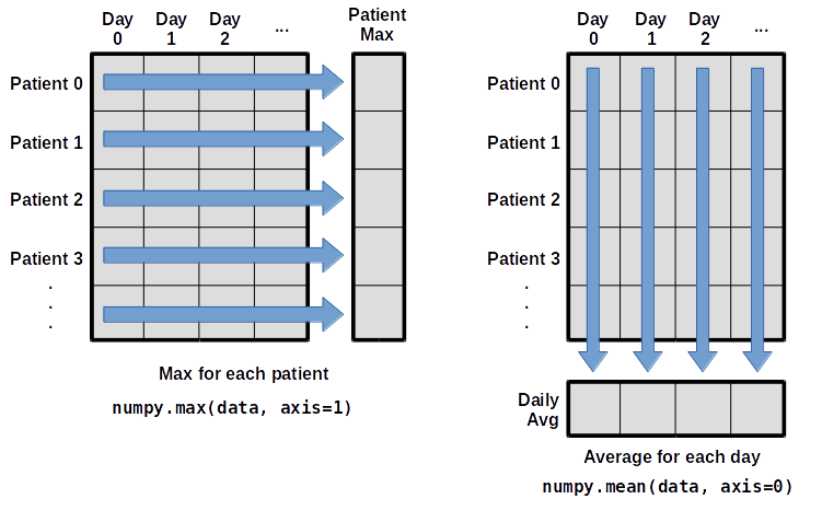
To find the maximum inflammation reported for each patient, you would apply the max function moving across the columns (axis 1). To find the daily average inflammation reported across patients, you would apply the mean function moving down the rows (axis 0).

To support this functionality, most array functions allow us to specify the axis we want to work on. If we ask for the max across axis 1 (columns in our 2D example), we get:

PYTHON

print(numpy.max(data, axis=1))

OUTPUT

[18. 18. 19. 17. 17. 18. 17. 20. 17. 18. 18. 18. 17. 16. 17. 18. 19. 19.
 17. 19. 19. 16. 17. 15. 17. 17. 18. 17. 20. 17. 16. 19. 15. 15. 19. 17.
 16. 17. 19. 16. 18. 19. 16. 19. 18. 16. 19. 15. 16. 18. 14. 20. 17. 15.
 17. 16. 17. 19. 18. 18.]

As a quick check, we can ask this array what its shape is. We expect 60 patient maximums:

PYTHON

print(numpy.max(data, axis=1).shape)

OUTPUT

(60,)

The expression (60,) tells us we have a one-dimensional array of 60 values. This data holds the maximum inflammation recorded for each patient.

If we ask for the average across/down axis 0 (rows in our 2D example), we get:

PYTHON

print(numpy.mean(data, axis=0))

OUTPUT

[ 0.          0.45        1.11666667  1.75        2.43333333  3.15
  3.8         3.88333333  5.23333333  5.51666667  5.95        5.9
  8.35        7.73333333  8.36666667  9.5         9.58333333 10.63333333
 11.56666667 12.35       13.25       11.96666667 11.03333333 10.16666667
 10.          8.66666667  9.15        7.25        7.33333333  6.58333333
  6.06666667  5.95        5.11666667  3.6         3.3         3.56666667
  2.48333333  1.5         1.13333333  0.56666667]

Check the array shape. We expect 40 averages, one for each day of the study:

PYTHON

print(numpy.mean(data, axis=0).shape)

OUTPUT

(40,)

Similarly, we can apply the mean function to axis 1 to get the patients’ average inflammation over the duration of the study (60 values).

PYTHON

print(numpy.mean(data, axis=1))

OUTPUT

[5.45  5.425 6.1   5.9   5.55  6.225 5.975 6.65  6.625 6.525 6.775 5.8
 6.225 5.75  5.225 6.3   6.55  5.7   5.85  6.55  5.775 5.825 6.175 6.1
 5.8   6.425 6.05  6.025 6.175 6.55  6.175 6.35  6.725 6.125 7.075 5.725
 5.925 6.15  6.075 5.75  5.975 5.725 6.3   5.9   6.75  5.925 7.225 6.15
 5.95  6.275 5.7   6.1   6.825 5.975 6.725 5.7   6.25  6.4   7.05  5.9  ]

Challenge

Slicing Strings

A section of an array is called a slice. We can take slices of character strings as well:

PYTHON

element = 'oxygen'
print('first three characters:', element[0:3])
print('last three characters:', element[3:6])

OUTPUT

first three characters: oxy
last three characters: gen

What is the value of element[:4]? What about element[4:]? Or element[:]?

Show me the solution

OUTPUT

oxyg
en
oxygen

Challenge

Slicing Strings (continued)

What is element[-1]? What is element[-2]?

Show me the solution

OUTPUT

n
e

Challenge

Slicing Strings (continued)

Given those answers, explain what element[1:-1] does.

Show me the solution

Creates a substring from index 1 up to (not including) the final index, effectively removing the first and last letters from ‘oxygen’

Challenge

Slicing Strings (continued)

How can we rewrite the slice for getting the last three characters of element, so that it works even if we assign a different string to element? Test your solution with the following strings: carpentry, clone, hi.

Show me the solution

PYTHON

element = 'oxygen'
print('last three characters:', element[-3:])
element = 'carpentry'
print('last three characters:', element[-3:])
element = 'clone'
print('last three characters:', element[-3:])
element = 'hi'
print('last three characters:', element[-3:])

OUTPUT

last three characters: gen
last three characters: try
last three characters: one
last three characters: hi

Pandas

---

Pandas is a Python library for data manipulation and analysis, providing powerful data structures like DataFrame and Series along with a wide range of functions for tasks such as data cleaning, preparation, and exploration. It is widely used in data science and machine learning workflows for its ease of use and flexibility.

We will now use the Iris dataset as an example of a dataset that does not just consist of numbers. This allows us to demonstrate some of the strengths of the Pandas library for inspecting structure and contents. To read in the dataset:

PYTHON

import pandas as pd

PYTHON

iris_df = pd.read_csv("../iris.csv")

Inspecting a Dataset

To understand the structure of the Iris dataset, we can use various methods provided by Pandas:

PYTHON

print(iris_df.head())

PYTHON

print(iris_df.info())

PYTHON

print(iris_df.describe())

Understanding the contents and data types of a dataset is important for accurate analysis.

Manipulating DataFrames

Pandas provides powerful functionalities to manipulate DataFrames. Here are some examples:

Adding and Removing Columns

Adding:

PYTHON

iris_df['sepal.ratio'] = iris_df['sepal.length'] / iris_df['sepal.width']

Removing:

PYTHON

iris_df.drop('variety', axis=1, inplace=True)

Adding and removing rows

Adding:

PYTHON

new_row = {'sepal.length': 5.1, 'sepal.width': 3.5, 'petal.length': 1.4, 'petal.width': 0.2,}
iris_df.loc[len(iris_df)] = new_row

Removing:

PYTHON

iris_df.drop(0, inplace=True)
iris_df.reset_index(drop=True, inplace=True)

Subsetting Data

Subsetting allows us to select specific rows or columns based on conditions:

PYTHON

iris_df = pd.read_csv("data/iris.csv") # reset the dataset
# Select rows where 'petal.length' is greater than 5
subset_df = iris_df[iris_df['petal.length'] > 5]

PYTHON

# Select rows where 'variety' is 'Setosa' and 'petal.length' is less than 1.5
subset_df = iris_df[(iris_df['variety'] == 'Setosa') & (iris_df['petal.length'] < 1.5)]

Key Points

• Remember array indices start at 0, not 1.
• Remember low:high to specify a slice that includes the indices from low to high-1.
• It’s good practice, especially when you are starting out, to use comments such as # explanation to explain what you are doing.
• We have shown some simple examples but you could slice your data in much more complicated ways depending on your requirements.
• It is hard to get an understanding of the data by just reading the raw numbers.

Content from Visualising Tabular Data

---

Last updated on 2026-04-01 | Edit this page

Estimated time: 60 minutes

Overview

Questions

• How can I visualise tabular data in Python?
• How can I generate several plots together?

Objectives

• Plot simple graphs from data.
• Plot multiple graphs in a single figure.

Visualizing data

---

The mathematician Richard Hamming once said, “The purpose of computing is insight, not numbers,” and the best way to develop insight is often to visualise data. Visualisation could take an entire course of its own, but for now we can explore a few features of Python’s matplotlib library here. While there is no official plotting library, matplotlib is the de facto standard. First, we will import the pyplot module from matplotlib and use two of its functions to create and display a heat map of our data:

Prerequisite

Episode Prerequisites

If you are continuing in the same notebook from the previous episode, you already have a data variable and have imported numpy. If you are starting a new notebook at this point, you need the following two lines:

PYTHON

import numpy as np
data = np.loadtxt(fname='../data/inflammation-01.csv', delimiter=',')

PYTHON

# you may need to %pip install matplotlib
import matplotlib.pyplot as plt
image = plt.imshow(data)
cbar = plt.colorbar()
plt.show()

Each row in the heat map corresponds to a patient in the clinical trial dataset, and each column corresponds to a day in the dataset. Blue pixels in this heat map represent low values, while yellow pixels represent high values. As we can see, the general number of inflammation flare-ups for the patients rises and falls over a 40-day period.

So far so good as this is in line with our knowledge of the clinical trial and Dr. Maverick’s claims:

• the patients take their medication once their inflammation flare-ups begin
• it takes around 3 weeks for the medication to take effect and begin reducing flare-ups
• and flare-ups appear to drop to zero by the end of the clinical trial.

Now let’s take a look at the average inflammation over time:

PYTHON

ave_inflammation = numpy.mean(data, axis=0)
ave_plot = plt.plot(ave_inflammation)
plt.show()

Here, we have put the average inflammation per day across all patients in the variable ave_inflammation, then asked matplotlib.pyplot to create and display a line graph of those values. The result is a reasonably linear rise and fall, in line with Dr. Maverick’s claim that the medication takes 3 weeks to take effect. But a good data scientist doesn’t just consider the average of a dataset, so let’s have a look at two other statistics:

PYTHON

max_plot = plt.plot(numpy.amax(data, axis=0))
plt.show()

PYTHON

min_plot = plt.plot(numpy.amin(data, axis=0))
plt.show()

The maximum value rises and falls linearly, while the minimum seems to be a step function. Neither trend seems particularly likely, so it’s likely there is something wrong with Dr Maverick’s data. This insight would have been difficult to reach by examining the numbers themselves without visualisation tools.

Grouping plots

You can group similar plots in a single figure using subplots. The script below uses a number of new commands. The function matplotlib.pyplot.figure() creates a figure into which we will place all of our plots. The parameter figsize tells Python how big to make this space. Each subplot is placed into the figure using its add_subplot method. The add_subplot method takes three parameters. The first denotes how many total rows of subplots there are, the second parameter refers to the total number of subplot columns, and the final parameter denotes which subplot your variable is referencing (left-to-right, top-to-bottom). Each subplot is stored in a different variable (axes1, axes2, axes3). Once a subplot is created, the axes can be titled using the set_xlabel() command (or set_ylabel()). Here are our three plots side by side:

PYTHON

data = numpy.loadtxt(fname='../data/inflammation-01.csv', delimiter=',')

fig = plt.figure(figsize=(10.0, 3.0))

axes1 = fig.add_subplot(1, 3, 1)
axes2 = fig.add_subplot(1, 3, 2)
axes3 = fig.add_subplot(1, 3, 3)

axes1.set_ylabel('average')
axes1.plot(numpy.mean(data, axis=0))

axes2.set_ylabel('max')
axes2.plot(numpy.amax(data, axis=0))

axes3.set_ylabel('min')
axes3.plot(numpy.amin(data, axis=0))

fig.tight_layout()

plt.savefig('inflammation.png')
plt.show()

The call to loadtxt reads our data, and the rest of the program tells the plotting library how large we want the figure to be, that we’re creating three subplots, what to draw for each one, and that we want a tight layout. (If we leave out that call to fig.tight_layout(), the graphs will actually be squeezed together more closely.)

The call to savefig stores the figure as a graphics file. This can be a convenient way to store your plots for use in other documents, web pages etc. The graphics format is automatically determined by Matplotlib from the file name ending we specify; here PNG from ‘inflammation.png’. Matplotlib supports many different graphics formats, including SVG, PDF, and JPEG.

Matplotlib cheatsheet 1 Matplotlib cheatsheet 2

Key Points

• We can easily visualise data using matplotlib.
• There are other libraries that are popular (e.g., seaborn).
• Getting figures “paper ready” can take a bit of time and effort.

Content from Flow control

---

Last updated on 2026-03-31 | Edit this page

Estimated time: 90 minutes

Overview

Questions

• How can I do the same operations on many different values?
• How can my programs do different things based on data values?

Objectives

• Explain what a for loop does.
• Correctly write for loops to repeat simple calculations.
• Write conditional statements including if, elif, and else branches.
• Correctly evaluate expressions containing and and or.

Often, we want to perform different operations in our code based upon dynamic conditions. To explore this idea, we are going to pretend we have two sensors. The first represents temperature, and the second represents if there is rainfall or not. Our temperature value is numeric, and the rainfall variable is a boolean. To declare those variables, you can type:

PYTHON

temp_reading = 16 

rainfall = True 

Then place the following code into your script:

PYTHON

if rainfall == True: 
  print("Advise user to take an umbrella") 

Run the script using the run button (little green play button) above the script pane.

PYTHON

Advise user to take an umbrella

From observing the output in the console and from a brief inspection of the code, it should be evident that we are evaluating the variable rainfall. Specifically, we are checking if it is True. If the outcome is of the check is true, then we perform any code within the indented block.

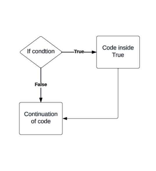
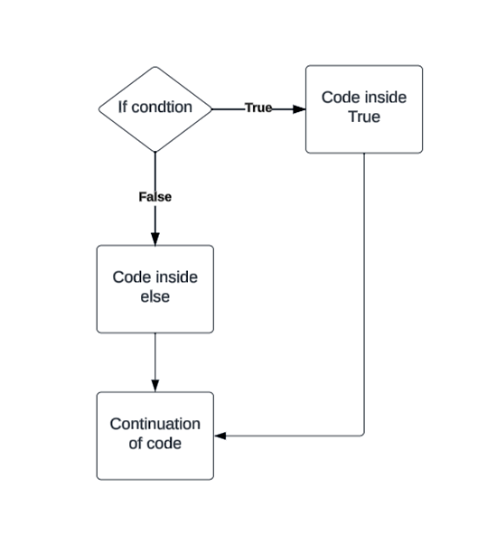
if, else

Now modify your code to look like this:

PYTHON

if rainfall: 
  print("Advise user to take an umbrella") 
else: 
  print("Leave your umbrella at home") 

Note: With boolean variables, we don’t actually have to write == True.

Change the condition

Now change the rainfall variable to False and run the script again.

PYTHON

rainfall = False

PYTHON

Leave your umbrella at home

Our code now reacts differently to different input values. You can combine if, elif (else if), and else statements to control the flow of your code.

Conditional statements

• ‘if’ – Runs a block of code if a condition is true.
• ‘elif’ – Checks another condition if the previous if or elif condition was false.
• ‘else’ – Runs a block of code if none of the previous conditions were true.

Comparison operators

We have encountered ‘==’, which is used to check for equivalence. There are other comparison operators available to us.

• > Greater than
• >= Greater than or equal to
• < Less than
• <= Less than or equal to
• == Equal to
• != Not equal to

Boolean operators

• and: Returns True only if both conditions are True.
• or: Returns True if at least one condition is True.
• not: Reverses a Boolean value, turning True into False and False into True.

Next:

PYTHON

if rainfall or temp_reading < 10:
    print("Stay at home") 
else:
    print("Go outside")

By combining these operators, you can create sophisticated flow control mechanisms.

For loops

In Python, a for loop is used to iterate over a sequence and perform a set of statements for each item in the sequence. Here is an example of a for loop in Python:

1. Syntax: The syntax of a for loop in Python is as follows:

   PYTHON

   for item in sequence:
       # Statements to execute for each item

2. Explanation:

   • The for keyword is used to start the loop.
   • item is a variable that takes each value from the sequence in each iteration of the loop.
   • sequence is the collection of items over which the loop iterates.
   • Indentation is used to define the block of statements to be executed for each iteration of the loop.

3. Examples: Here’s an examples of a for loop that iterates over a range of numbers and prints each number:

PYTHON

   for i in range(5):
       print(i)

{: .language.python}

PYTHON

0
1
2
3
4

Here’s an examples of a for loop that iterates over a list of strings and prints each string:

PYTHON

days = ['monday','tuesday','wednesday','thursday','friday']

for day in days:
    print(day)

PYTHON

monday
tuesday
wednesday
thursday
friday

For loops are commonly used in Python for iterating over sequences, performing repetitive tasks, and processing collections of data.

Keeping things clear

It is possible to put conditional statements inside conditional statements these are then referred to as ‘nested’. If your code becomes overly nested it can impact readability and maintainability. It is good practice to keep your workflow as simple as possible, this can be made easier by spending time on design and regular refactoring.

Note: Refactoring is the process of restructuring code, not to change the functionality but to improve factors like readability, maintainability, efficiency.

We’ve covered a very basic introduction to flow control in Python, but there are many more facets to explore in order to fully understand all possibilities. Please feel free to check out the link below for more information on flow control.

Python control flow tutorial

Key Points

• Use for variable in sequence to process the elements of a sequence one at a time.
• Don’t forget to indent.
• You can use len(thing) to determine the length of something that contains other values.
• Use if condition to start a conditional statement, elif condition to provide additional tests, and else to provide a default.
• Use == to test for equality and = for assignment.
• In Python, some values are treated as false in conditions, including \0, '', [], and None.

Content from Creating Functions

---

Last updated on 2026-03-31 | Edit this page

Estimated time: 90 minutes

Overview

Questions

• How can I define new functions?
• What’s the difference between defining and calling a function?
• What happens when I call a function?
• Why do I need functions?

Objectives

• Define a function that takes parameters.
• Return a value from a function.
• Test and debug a function.
• Set default values for function parameters.
• Explain why we should divide programs into small, single-purpose functions.

At this point, we’ve seen that code can have Python make decisions about what it sees in our data. What if we want to convert some of our data, like taking a temperature in Fahrenheit and converting it to Celsius. We could write something like this for converting a single number

PYTHON

fahrenheit_val = 99
celsius_val = ((fahrenheit_val - 32) * (5/9))

and for a second number we could just copy the line and rename the variables

PYTHON

fahrenheit_val = 99
celsius_val = ((fahrenheit_val - 32) * (5/9))

fahrenheit_val2 = 43
celsius_val2 = ((fahrenheit_val2 - 32) * (5/9))

But we would be in trouble as soon as we had to do this more than a couple times. Cutting and pasting it is going to make our code get very long and very repetitive, very quickly. We’d like a way to package our code so that it is easier to reuse, a shorthand way of re-executing longer pieces of code. In Python we can use ‘functions’. Let’s start by defining a function fahr_to_celsius that converts temperatures from Fahrenheit to Celsius:

PYTHON

def explicit_fahr_to_celsius(temp):
    # Assign the converted value to a variable
    converted = ((temp - 32) * (5/9))
    # Return the value of the new variable
    return converted
    
def fahr_to_celsius(temp):
    # Return converted value more efficiently using return
    # without creating a new variable. This code does
    # the same thing as the previous function but in a shorter way.
    return ((temp - 32) * (5/9))

The function definition opens with the keyword def followed by the name of the function (fahr_to_celsius) and a parenthesized list of parameter names (temp). The body of the function, the statements that are executed when it runs, is indented below the definition line. The body concludes with a return keyword followed by the return value.

When we call the function, the values we pass to it are assigned to those variables so that we can use them inside the function. Inside the function, we use a return statement to send a result back to whoever asked for it.

Let’s try running our function.

PYTHON

fahr_to_celsius(32)

This command should call our function, using “32” as the input and return the function value.

In fact, calling our own function is no different from calling any other function:

PYTHON

print('freezing point of water:', fahr_to_celsius(32), 'C')
print('boiling point of water:', fahr_to_celsius(212), 'C')

OUTPUT

freezing point of water: 0.0 C
boiling point of water: 100.0 C

We’ve successfully called the function that we defined, and we have access to the value that we returned.

Composing Functions

---

Now that we’ve seen how to turn Fahrenheit into Celsius, we can also write the function to turn Celsius into Kelvin:

PYTHON

def celsius_to_kelvin(temp_c):
    return temp_c + 273.15

print('freezing point of water in Kelvin:', celsius_to_kelvin(0.))

OUTPUT

freezing point of water in Kelvin: 273.15

What about converting Fahrenheit to Kelvin? We could write out the formula, but we don’t need to. Instead, we can compose the two functions we have already created:

PYTHON

def fahr_to_kelvin(temp_f):
    temp_c = fahr_to_celsius(temp_f)
    temp_k = celsius_to_kelvin(temp_c)
    return temp_k

print('boiling point of water in Kelvin:', fahr_to_kelvin(212.0))

OUTPUT

boiling point of water in Kelvin: 373.15

This is our first taste of how larger programs are built: we define basic operations, then combine them in ever-larger chunks to get the effect we want. In practice, many functions are longer than the ones shown here, but it is usually a good idea to keep functions focused on a single task and not make them unnecessarily long.

Variable Scope

---

In composing our temperature conversion functions, we created variables inside of those functions, temp, temp_c, temp_f, and temp_k. We refer to these variables as local variables because they no longer exist once the function is done executing. If we try to access their values outside of the function, we will encounter an error:

PYTHON

print('Again, temperature in Kelvin was:', temp_k)

ERROR

---------------------------------------------------------------------------
NameError                                 Traceback (most recent call last)
<ipython-input-1-eed2471d229b> in <module>
----> 1 print('Again, temperature in Kelvin was:', temp_k)

NameError: name 'temp_k' is not defined

If you want to reuse the temperature in Kelvin after you have calculated it with fahr_to_kelvin, you can store the result of the function call in a variable:

PYTHON

temp_kelvin = fahr_to_kelvin(212.0)
print('temperature in Kelvin was:', temp_kelvin)

OUTPUT

temperature in Kelvin was: 373.15

The variable temp_kelvin, being defined outside any function, is said to be global.

Inside a function, one can read the value of such global variables:

PYTHON

def print_temperatures():
    print('temperature in Fahrenheit was:', temp_fahr)
    print('temperature in Kelvin was:', temp_kelvin)

temp_fahr = 212.0
temp_kelvin = fahr_to_kelvin(temp_fahr)

print_temperatures()

OUTPUT

temperature in Fahrenheit was: 212.0
temperature in Kelvin was: 373.15

Although a function can read values from global variables, relying too much on globals can make code harder to understand and test, therefore best practice is to avoid this.

Tidying up

---

Now that we know how to wrap bits of code up in functions, we can make our inflammation analysis easier to read and easier to reuse. First, let’s make a visualize function that generates our plots:

PYTHON

def visualize(filename):

    data = np.loadtxt(fname=filename, delimiter=',')

    fig = plt.figure(figsize=(10.0, 3.0))

    axes1 = fig.add_subplot(1, 3, 1)
    axes2 = fig.add_subplot(1, 3, 2)
    axes3 = fig.add_subplot(1, 3, 3)

    axes1.set_ylabel('average')
    axes1.plot(np.mean(data, axis=0))

    axes2.set_ylabel('max')
    axes2.plot(np.amax(data, axis=0))

    axes3.set_ylabel('min')
    axes3.plot(np.amin(data, axis=0))

    fig.tight_layout()
    plt.show()

and another function called detect_problems that checks for those suspicious patterns we noticed:

PYTHON

def detect_problems(filename):

    data = np.loadtxt(fname=filename, delimiter=',')

    if np.amax(data, axis=0)[0] == 0 and np.amax(data, axis=0)[20] == 20:
        print('Suspicious looking maxima!')
    elif np.sum(np.amin(data, axis=0)) == 0:
        print('Minima add up to zero!')
    else:
        print('Seems OK!')

Wait! Didn’t we forget to specify what both of these functions should return? Well, we didn’t. In Python, functions are not required to include a return statement and can be used for the sole purpose of grouping together pieces of code that conceptually do one thing. In such cases, function names usually describe what they do, e.g. visualize, detect_problems. Where no return is included, as a default, Python will return a none.

Notice that rather than jumbling this code together in one giant for loop, we can now read and reuse both ideas separately. We can reproduce the previous analysis with a much simpler for loop:

PYTHON

filenames = sorted(glob.glob('../data/inflammation*.csv'))

for filename in filenames[:3]:
    print(filename)
    visualize(filename)
    detect_problems(filename)

By giving our functions human-readable names, we can more easily read and understand what is happening in the for loop. Even better, if at some later date we want to use either of those pieces of code again, we can do so in a single line.

Testing and Documenting

---

Once we start putting things in functions so that we can re-use them, it is good practice to write some documentation to remind ourselves later what it’s for and how to use it.

If the first thing in a function is a string that isn’t assigned to a variable, that string is attached to the function as its documentation:

PYTHON

def visualize(filename):
    """Load a CSV file and plot the average, maximum, and minimum values for each day."""
    

A string like this is called a docstring. Docstrings are usually written with triple quotes, which also lets us spread them across multiple lines if needed:

PYTHON

def visualize(filename):
    """
    Load inflammation data from a CSV file and display three summary plots.

    This function reads numerical data from the file given by `filename`,
    where each row represents one patient and each column represents one day.
    It then creates a figure with three side-by-side line plots showing:

    1. The average value for each day across all patients.
    2. The maximum value for each day across all patients.
    3. The minimum value for each day across all patients.

    Parameters
    ----------
    filename : str
        The path to the CSV file containing the inflammation data.

    Returns
    -------
    None

    """

Defining Defaults

---

We have passed parameters to functions in two ways: directly, as in type(data), and by name, as in np.loadtxt(fname='something.csv', delimiter=','). In fact, we can pass the filename to loadtxt without the fname=:

PYTHON

np.loadtxt('../data/inflammation-01.csv', delimiter=',')

OUTPUT

array([[ 0.,  0.,  1., ...,  3.,  0.,  0.],
       [ 0.,  1.,  2., ...,  1.,  0.,  1.],
       [ 0.,  1.,  1., ...,  2.,  1.,  1.],
       ...,
       [ 0.,  1.,  1., ...,  1.,  1.,  1.],
       [ 0.,  0.,  0., ...,  0.,  2.,  0.],
       [ 0.,  0.,  1., ...,  1.,  1.,  0.]])

but we still need to say delimiter=:

PYTHON

np.loadtxt('../data/inflammation-01.csv', ',')

ERROR

Traceback (most recent call last):
  File "<stdin>", line 1, in <module>
  File "/Users/username/anaconda3/lib/python3.6/site-packages/numpy/lib/npyio.py", line 1041, in loa
dtxt
    dtype = np.dtype(dtype)
  File "/Users/username/anaconda3/lib/python3.6/site-packages/numpy/core/_internal.py", line 199, in
_commastring
    newitem = (dtype, eval(repeats))
  File "<string>", line 1
    ,
    ^
SyntaxError: unexpected EOF while parsing

Let’s look at the help for np.loadtxt:

PYTHON

help(np.loadtxt)

OUTPUT

Help on function loadtxt in module np.lib.npyio:

loadtxt(fname, dtype=<class 'float'>, comments='#', delimiter=None, converters=None, skiprows=0, use
cols=None, unpack=False, ndmin=0, encoding='bytes')
    Load data from a text file.

    Each row in the text file must have the same number of values.

    Parameters
    ----------
...

There’s a lot of information here, but the most important part is the first couple of lines:

OUTPUT

loadtxt(fname, dtype=<class 'float'>, comments='#', delimiter=None, converters=None, skiprows=0, use
cols=None, unpack=False, ndmin=0, encoding='bytes')

This tells us that loadtxt has one parameter called fname that doesn’t have a default value, and eight others that do. If we call the function like this:

PYTHON

np.loadtxt('../data/inflammation-01.csv', ',')

then the filename is assigned to fname (which is what we want), but the delimiter string ',' is assigned to dtype rather than delimiter, because dtype is the second parameter in the list. However ',' isn’t a known dtype so our code produced an error message when we tried to run it. When we call loadtxt we don’t have to provide fname= for the filename because it’s the first item in the list, but if we want the ',' to be assigned to the variable delimiter, we do have to provide delimiter= for the second parameter since delimiter is not the second parameter in the list.

If we usually want a function to work one way, but occasionally need it to do something else, we can allow people to pass a parameter when they need to but provide a default to make the normal case easier. The example below shows how Python matches values to parameters:

PYTHON

def display(a=1, b=2, c=3):
    print('a:', a, 'b:', b, 'c:', c)

print('no parameters:')
display()
print('one parameter:')
display(55)
print('two parameters:')
display(55, 66)

OUTPUT

no parameters:
a: 1 b: 2 c: 3
one parameter:
a: 55 b: 2 c: 3
two parameters:
a: 55 b: 66 c: 3

As this example shows, parameters are matched up from left to right, and any that haven’t been given a value explicitly get their default value. We can override this behavior by naming the value as we pass it in:

PYTHON

print('only setting the value of c')
display(c=77)

OUTPUT

only setting the value of c
a: 1 b: 2 c: 77

Readable functions

---

Consider these two functions:

PYTHON

def s(p):
    a = 0
    for v in p:
        a += v
    m = a / len(p)
    d = 0
    for v in p:
        d += (v - m) * (v - m)
    return np.sqrt(d / (len(p) - 1))

def std_dev(sample):
    sample_sum = 0
    for value in sample:
        sample_sum += value

    sample_mean = sample_sum / len(sample)

    sum_squared_devs = 0
    for value in sample:
        sum_squared_devs += (value - sample_mean) * (value - sample_mean)

    return np.sqrt(sum_squared_devs / (len(sample) - 1))

The functions s and std_dev are computationally equivalent (they both calculate the sample standard deviation), but to a human reader, they look very different. You probably found std_dev much easier to read and understand than s.

As this example illustrates, both documentation and a programmer’s coding style combine to determine how easy it is for others to read and understand the programmer’s code. Choosing meaningful variable names and using blank spaces to break the code into logical “chunks” are helpful techniques for producing readable code. This is useful not only for sharing code with others, but also for the original programmer. If you need to revisit code that you wrote months ago and haven’t thought about since then, you will appreciate the value of readable code!

Challenges

---

Challenge

Combining Strings

“Adding” two strings produces their concatenation: 'a' + 'b' is 'ab'. Write a function called fence that takes two parameters called original and wrapper and returns a new string that has the wrapper character at the beginning and end of the original. A call to your function should look like this:

PYTHON

print(fence('name', '*'))

OUTPUT

*name*

Show me the solution

PYTHON

def fence(original, wrapper):
    return wrapper + original + wrapper

Challenge

Variables Inside and Outside Functions

What does the following piece of code display when run — and why?

PYTHON

f = 0
k = 0

def f2k(f):
    k = ((f - 32) * (5.0 / 9.0)) + 273.15
    return k

print(f2k(8))
print(f2k(41))
print(f2k(32))

print(k)

Show me the solution

OUTPUT

259.81666666666666
278.15
273.15
0

k is 0 because the k inside the function f2k doesn’t know about the k defined outside the function. When the f2k function is called, it creates a local variable k. The function returns a local k but that does not alter the k outside of its local copy. Therefore the original value of k remains unchanged. Beware that a local k is created because f2k internal statements affect a new value to it. If k was only read, it would simply retrieve the global k value.

Key Points

• The body of a function must be indented.
• The scope of variables defined within a function can only be seen and used within the body of the function.
• Variables created outside of any function are called global variables.
• Within a function, we can access global variables.
• Variables created within a function override global variables if their names match.
• Put docstrings in functions to provide help for that function.
• Specify default values for parameters when defining a function using name=value in the parameter list.
• Parameters can be passed by matching based on name, by position, or by omitting them (in which case the default value is used).
• Put code whose parameters change frequently in a function, then call it with different parameter values to customize its behavior.

Content from Pathing and workspaces

---

Last updated on 2026-03-31 | Edit this page

Estimated time: 60 minutes

Overview

Questions

• How do I know what Python can “see”?
• Where am I working?
• Where are my outputs going?

Objectives

• explain where a notebook is stored
• explain where data files are stored
• use relative paths
• load a CSV file
• load an image file
• load an audio file
• spot and fix common file and path mistakes

Files, Folders, and Paths

---

What are files, folders, and paths?

A file is a single item stored on a computer, such as:

• a notebook
• a CSV file
• an image
• an audio file

A folder contains files and sometimes other folders.

A path is the set of directions that tells the computer where a file is located in the folder structure. A path identifies an item in a hierarchical file system.

Analogy

Think of a computer like a building:

• folders are rooms
• files are objects inside the rooms
• a path is the directions to reach one object

For example:

PYTHON

project/data/sales.csv

This means:

• go to the project folder
• then the data folder
• then find the file sales.csv

Where is the notebook?

A Jupyter notebook is itself a file, usually ending in .ipynb.

That means the notebook lives in a folder somewhere on your computer, just like any other file. In Jupyter, the notebook runs relative to a current working directory, and relative paths depend on that location.

Important idea

When you write code to open a file, Python needs to know:

“Starting from where?”

Usually, that starting point is the current working directory, which is often the same as the notebook’s folder.

So if your notebook is in:

PYTHON

project/
    analysis.ipynb

then the notebook is inside the project folder.

Where is the data?

Your data is stored as separate files somewhere in your folders.

For example:

PYTHON

project/
    analysis.ipynb
    data/
        sales.csv
        cat.jpg
        song.wav

Here:

• the notebook is analysis.ipynb
• the data files are inside the data folder

This is a very common and sensible structure because it keeps the notebook and data organised. Good project structure makes work easier to repeat and understand.

Relative paths

A relative path gives directions from the current notebook location, rather than from the very top of the computer. Relative paths assume you are starting in the current working directory.

Example folder structure

PYTHON

project/
    notebook.ipynb
    data/
        marks.csv

If the notebook is in project/ and the file is inside data/, the relative path is:

PYTHON

"data/marks.csv"

This means:

• from where the notebook is now
• go into the data folder
• open marks.csv

Why relative paths are useful

Relative paths are better for classwork and projects because:

• they are shorter
• they are easier to read
• they work better when a project folder is moved to another computer

Some additional file types

---

Loading an image

One common way to load an image is with PIL:

PYTHON

from PIL import Image

img = Image.open("../additional_stuff/cat.jpg")
img.show()

This opens the image file from the data folder.

You can also use a library called OpenCV.

PYTHON

import cv2

img = cv2.imread("../additional_stuff/cat.jpg")
cv2.imshow("Image", img)
cv2.waitKey(0)
cv2.destroyAllWindows()

Another common option in notebooks is matplotlib:

PYTHON

import matplotlib.pyplot as plt
import matplotlib.image as mpimg

img = mpimg.imread("../additional_stuff/cat.jpg")
plt.imshow(img)
plt.axis("off")

Loading an audio file

A simple notebook-friendly way is to use IPython display tools:

PYTHON

from IPython.display import Audio

filename = "../additional_stuff/03-01-01-01-01-02-01.wav"
Audio(filename)

This loads the audio file and gives you a player in the notebook.

We can visualise the audio using tools we have already encountered and a new libraries (scipy).

PYTHON

from scipy.io import wavfile

sample_rate, data = wavfile.read(filename)

plt.figure(figsize=(10, 3))
plt.plot(data)
plt.ylabel("Amplitude")
plt.show()

Troubleshooting / debugging path problems

When a file will not load, students should ask:

• Where is my notebook?
• Where is my file?
• What path am I giving Python?
• Is the filename spelled correctly?
• Is the extension correct?
• Am I using the right folder names?

A helpful debugging command is:

PYTHON

import os
print(os.getcwd())
print(os.listdir())

This shows:

• the current folder
• the files and folders inside it

Key Points

• Be aware of your current working directory
• One of the biggest struggle for importing your data into Python is getting the paths correct.

Content from Errors and Exceptions

---

Last updated on 2026-03-31 | Edit this page

Estimated time: 60 minutes

Overview

Questions

• How does Python report errors?
• How can I handle errors in Python programs?
• How can I debug my program?

Objectives

• To be able to read a traceback, and determine where the error took place and what type of error we are dealing with.
• Be aware of different types of errors (e.g. indentation errors and name errors).
• Understand the process of debugging code containing an error systematically.
• Identify ways of making code less error-prone and more easily tested.

Every programmer encounters errors, both those who are just beginning, and those who have been programming for years. Encountering errors and exceptions can be very frustrating at times, and can make coding feel like a hopeless endeavour. However, understanding what the different types of errors are and when you are likely to encounter them can help a lot. Once you know why you get certain types of errors, they become much easier to fix.

Errors in Python have a very specific form, called a traceback. Let’s examine one:

PYTHON

# This code has an intentional error. You can type it directly or
# use it for reference to understand the error message below.
def favorite_ice_cream():
    ice_creams = [
        'chocolate',
        'vanilla',
        'strawberry'
    ]
    print(ice_creams[3])

favorite_ice_cream()

ERROR

---------------------------------------------------------------------------
IndexError                                Traceback (most recent call last)
<ipython-input-1-70bd89baa4df> in <module>()
      9     print(ice_creams[3])
      10
----> 11 favorite_ice_cream()

<ipython-input-1-70bd89baa4df> in favorite_ice_cream()
      7         'strawberry'
      8     ]
----> 9     print(ice_creams[3])
      10
      11 favorite_ice_cream()

IndexError: list index out of range

This particular traceback has two levels. You can determine the number of levels by looking for the number of arrows on the left-hand side. In this case:

1. The first shows code from the cell above, with an arrow pointing to Line 11 (which is favorite_ice_cream()).

2. The second shows some code in the function favorite_ice_cream, with an arrow pointing to Line 9 (which is print(ice_creams[3])).

The last level is the actual place where the error occurred. The other level(s) show what function the program executed to get to the next level down. So, in this case, the program first performed a function call to the function favorite_ice_cream. Inside this function, the program encountered an error on Line 9, when it tried to run the code print(ice_creams[3]).

Callout

Long Tracebacks

Sometimes, you might see a traceback that is very long -- sometimes they might even be 20 levels deep! This can make it seem like something horrible happened, but the length of the error message does not reflect severity, rather, it indicates that your program called many functions before it encountered the error. Most of the time, the actual place where the error occurred is at the bottom-most level, so you can skip down the traceback to the bottom.

So what error did the program actually encounter? In the last line of the traceback, Python helpfully tells us the category or type of error (in this case, it is an IndexError) and a more detailed error message (in this case, it says “list index out of range”).

If you encounter an error and don’t know what it means, it is still important to read the traceback closely. That way, if you fix the error, but encounter a new one, you can tell that the error changed. Additionally, sometimes knowing where the error occurred is enough to fix it, even if you don’t entirely understand the message.

If you do encounter an error you don’t recognize, try looking at the official documentation on errors. However, note that you may not always be able to find the error there, as it is possible to create custom errors. In that case, hopefully the custom error message is informative enough to help you figure out what went wrong.

Callout

Better errors on newer versions of Python

Newer versions of Python have improved error printouts. If you are debugging errors, it is often helpful to use the latest Python version, even if you support older versions of Python.

Syntax Errors

---

When you forget a colon at the end of a line, accidentally add one space too many when indenting under an if statement, or forget a parenthesis, you will encounter a syntax error. This means that Python couldn’t figure out how to read your program. This is similar to forgetting punctuation in English: for example, this text is difficult to read there is no punctuation there is also no capitalisation why is this hard because you have to figure out where each sentence ends you also have to figure out where each sentence begins to some extent it might be ambiguous if there should be a sentence break or not

People can typically figure out what is meant by text with no punctuation, but people are much smarter than computers. If Python doesn’t know how to read the program, it will give up and inform you with an error. For example:

PYTHON

def some_function()
    msg = 'hello, world!'
    print(msg)
     return msg

ERROR

  File "<ipython-input-3-6bb841ea1423>", line 1
    def some_function()
                       ^
SyntaxError: invalid syntax

Here, Python tells us that there is a SyntaxError on line 1, and even puts a little arrow in the place where there is an issue. In this case the problem is that the function definition is missing a colon at the end.

Actually, the function above has two issues with syntax. If we fix the problem with the colon, we see that there is also an IndentationError, which means that the lines in the function definition do not all have the same indentation:

PYTHON

def some_function():
    msg = 'hello, world!'
    print(msg)
     return msg

ERROR

  File "<ipython-input-4-ae290e7659cb>", line 4
    return msg
    ^
IndentationError: unexpected indent

Both SyntaxError and IndentationError indicate a problem with the syntax of your program, but an IndentationError is more specific: it always means that there is a problem with how your code is indented.

Callout

Tabs and Spaces

Some indentation errors are harder to spot than others. In particular, mixing spaces and tabs can be difficult to spot because they are both whitespace. In the example below, the first two lines in the body of the function some_function are indented with tabs, while the third line — with spaces. If you’re working in a Jupyter notebook, be sure to copy and paste this example rather than trying to type it in manually because Jupyter automatically replaces tabs with spaces.

PYTHON

def some_function():
	msg = 'hello, world!'
	print(msg)
        return msg

Visually it is impossible to spot the error. Fortunately, Python does not allow you to mix tabs and spaces.

ERROR

  File "<ipython-input-5-653b36fbcd41>", line 4
    return msg
              ^
TabError: inconsistent use of tabs and spaces in indentation

Variable Name Errors

---

Another very common type of error is called a NameError, and occurs when you try to use a variable that does not exist. For example:

PYTHON

print(a)

ERROR

---------------------------------------------------------------------------
NameError                                 Traceback (most recent call last)
<ipython-input-7-9d7b17ad5387> in <module>()
----> 1 print(a)

NameError: name 'a' is not defined

Variable name errors come with some of the most informative error messages, which are usually of the form “name ‘the_variable_name’ is not defined”.

Why does this error message occur? That’s a harder question to answer, because it depends on what your code is supposed to do. However, there are a few very common reasons why you might have an undefined variable. The first is that you meant to use a string, but forgot to put quotes around it:

PYTHON

print(hello)

ERROR

---------------------------------------------------------------------------
NameError                                 Traceback (most recent call last)
<ipython-input-8-9553ee03b645> in <module>()
----> 1 print(hello)

NameError: name 'hello' is not defined

The second reason is that you might be trying to use a variable that does not yet exist. In the following example, count should have been defined (e.g., with count = 0) before the for loop:

PYTHON

for number in range(10):
    count = count + number
print('The count is:', count)

ERROR

---------------------------------------------------------------------------
NameError                                 Traceback (most recent call last)
<ipython-input-9-dd6a12d7ca5c> in <module>()
      1 for number in range(10):
----> 2     count = count + number
      3 print('The count is:', count)

NameError: name 'count' is not defined

Finally, the third possibility is that you made a typo when you were writing your code. Let’s say we fixed the error above by adding the line Count = 0 before the for loop. Frustratingly, this actually does not fix the error. Remember that variables are case-sensitive, so the variable count is different from Count. We still get the same error, because we still have not defined count:

PYTHON

Count = 0
for number in range(10):
    count = count + number
print('The count is:', count)

ERROR

---------------------------------------------------------------------------
NameError                                 Traceback (most recent call last)
<ipython-input-10-d77d40059aea> in <module>()
      1 Count = 0
      2 for number in range(10):
----> 3     count = count + number
      4 print('The count is:', count)

NameError: name 'count' is not defined

Index Errors

---

Next up are errors having to do with containers (like lists and strings) and the items within them. If you try to access an item in a list or a string that does not exist, then you will get an error. This makes sense: if you asked someone what day they would like to get coffee, and they answered “caturday”, you might be a bit annoyed. Python gets similarly annoyed if you try to ask it for an item that doesn’t exist:

PYTHON

letters = ['a', 'b', 'c']
print('Letter #1 is', letters[0])
print('Letter #2 is', letters[1])
print('Letter #3 is', letters[2])
print('Letter #4 is', letters[3])

OUTPUT

Letter #1 is a
Letter #2 is b
Letter #3 is c

ERROR

---------------------------------------------------------------------------
IndexError                                Traceback (most recent call last)
<ipython-input-11-d817f55b7d6c> in <module>()
      3 print('Letter #2 is', letters[1])
      4 print('Letter #3 is', letters[2])
----> 5 print('Letter #4 is', letters[3])

IndexError: list index out of range

Here, Python is telling us that there is an IndexError in our code, meaning we tried to access a list index that did not exist.

File Errors

---

The last type of error we’ll cover today are those associated with reading and writing files: FileNotFoundError. If you try to read a file that does not exist, you will receive a FileNotFoundError telling you so. If you attempt to write to a file that was opened read-only, Python 3 returns an UnsupportedOperationError. More generally, problems with input and output manifest as OSErrors, which may show up as a more specific subclass; you can see the list in the Python docs. They all have a unique UNIX errno, which is you can see in the error message.

PYTHON

file_handle = open('myfile.txt', 'r')

ERROR

---------------------------------------------------------------------------
FileNotFoundError                         Traceback (most recent call last)
<ipython-input-14-f6e1ac4aee96> in <module>()
----> 1 file_handle = open('myfile.txt', 'r')

FileNotFoundError: [Errno 2] No such file or directory: 'myfile.txt'

One reason for receiving this error is that you specified an incorrect path to the file. For example, if I am currently in a folder called myproject, and I have a file in myproject/writing/myfile.txt, but I try to open myfile.txt, this will fail. The correct path would be writing/myfile.txt. It is also possible that the file name or its path contains a typo.

A related issue can occur if you use the “read” flag instead of the “write” flag. Python will not give you an error if you try to open a file for writing when the file does not exist. However, if you meant to open a file for reading, but accidentally opened it for writing, and then try to read from it, you will get an UnsupportedOperation error telling you that the file was not opened for reading:

PYTHON

file_handle = open('myfile.txt', 'w')
file_handle.read()

ERROR

---------------------------------------------------------------------------
UnsupportedOperation                      Traceback (most recent call last)
<ipython-input-15-b846479bc61f> in <module>()
      1 file_handle = open('myfile.txt', 'w')
----> 2 file_handle.read()

UnsupportedOperation: not readable

These are the most common errors with files, though many others exist. If you get an error that you’ve never seen before, searching the Internet for that error type often reveals common reasons why you might get that error.

Once testing has uncovered problems, the next step is to fix them. Many novices do this by making more-or-less random changes to their code until it seems to produce the right answer, but that’s very inefficient (and the result is usually only correct for the one case they’re testing). The more experienced a programmer is, the more systematically they debug, and most follow some variation on the rules explained below.

Know What It’s Supposed to Do

---

The first step in debugging something is to know what it’s supposed to do. “My program doesn’t work” isn’t good enough: in order to diagnose and fix problems, we need to be able to tell correct output from incorrect. If we can write a test case for the failing case — i.e., if we can assert that with these inputs, the function should produce that result — then we’re ready to start debugging. If we can’t, then we need to figure out how we’re going to know when we’ve fixed things.

But writing test cases for scientific software is frequently harder than writing test cases for commercial applications, because if we knew what the output of the scientific code was supposed to be, we wouldn’t be running the software: we’d be writing up our results and moving on to the next program. In practice, scientists tend to do the following:

1. Test with simplified data. Before doing statistics on a real data set, we should try calculating statistics for a single record, for two identical records, for two records whose values are one step apart, or for some other case where we can calculate the right answer by hand.

2. Test a simplified case. If our program is supposed to simulate magnetic eddies in rapidly-rotating blobs of supercooled helium, our first test should be a blob of helium that isn’t rotating, and isn’t being subjected to any external electromagnetic fields. Similarly, if we’re looking at the effects of climate change on speciation, our first test should hold temperature, precipitation, and other factors constant.

3. Compare to an oracle. A test oracle is something whose results are trusted, such as experimental data, an older program, or a human expert. We use test oracles to determine if our new program produces the correct results. If we have a test oracle, we should store its output for particular cases so that we can compare it with our new results as often as we like without re-running that program.

4. Check conservation laws. Mass, energy, and other quantities are conserved in physical systems, so they should be in programs as well. Similarly, if we are analyzing patient data, the number of records should either stay the same or decrease as we move from one analysis to the next (since we might throw away outliers or records with missing values). If “new” patients start appearing out of nowhere as we move through our pipeline, it’s probably a sign that something is wrong.

5. Visualise. Data analysts frequently use simple visualisations to check both the science they’re doing and the correctness of their code (just as we did in the opening lesson of this tutorial). This should not be the only debugging method you rely on, since visual comparisons are hard to automate.

Make It Fail Every Time

---

We can only debug something when it fails, so the second step is always to find a test case that makes it fail every time. The “every time” part is important because few things are more frustrating than debugging an intermittent problem: if we have to call a function a dozen times to get a single failure, the odds are good that we’ll scroll past the failure when it actually occurs.

As part of this, it’s always important to check that our code is “plugged in”, i.e., that we’re actually exercising the problem that we think we are. Every programmer has spent hours chasing a bug, only to realize that they were actually calling their code on the wrong data set or with the wrong configuration parameters, or are using the wrong version of the software entirely. Mistakes like these are particularly likely to happen when we’re tired, frustrated, and up against a deadline, which is one of the reasons late-night (or overnight) coding sessions are almost never worthwhile.

Make It Fail Fast

---

If it takes 20 minutes for the bug to surface, we can only do three experiments an hour. This means that we’ll get less data in more time and that we’re more likely to be distracted by other things as we wait for our program to fail, which means the time we are spending on the problem is less focused. It’s therefore critical to make it fail fast.

As well as making the program fail fast in time, we want to make it fail fast in space, i.e., we want to localize the failure to the smallest possible region of code:

1. The smaller the gap between cause and effect, the easier the connection is to find. Many programmers therefore use a divide and conquer strategy to find bugs, i.e., if the output of a function is wrong, they check whether things are OK in the middle, then concentrate on either the first or second half, and so on.

2. N things can interact in N! different ways, so every line of code that isn’t run as part of a test means more than one thing we don’t need to worry about.

Change One Thing at a Time, For a Reason

---

Replacing random chunks of code is unlikely to do much good. (After all, if you got it wrong the first time, you’ll probably get it wrong the second and third as well.) Good programmers therefore change one thing at a time, for a reason. They are either trying to gather more information (“is the bug still there if we change the order of the loops?”) or test a fix (“can we make the bug go away by sorting our data before processing it?”).

Every time we make a change, however small, we should re-run our tests immediately, because the more things we change at once, the harder it is to know what’s responsible for what (those N! interactions again). And we should re-run all of our tests: more than half of fixes made to code introduce (or re-introduce) bugs, so re-running all of our tests tells us whether we have regressed.

Keep Track of What You’ve Done

---

Good scientists keep track of what they’ve done so that they can reproduce their work, and so that they don’t waste time repeating the same experiments or running ones whose results won’t be interesting. Similarly, debugging works best when we keep track of what we’ve done and how well it worked. If we find ourselves asking, “Did left followed by right with an odd number of lines cause the crash? Or was it right followed by left? Or was I using an even number of lines?” then it’s time to step away from the computer, take a deep breath, and start working more systematically.

Records are particularly useful when the time comes to ask for help. People are more likely to listen to us when we can explain clearly what we did, and we’re better able to give them the information they need to be useful.

Callout

Version Control Revisited

Version control is often used to reset software to a known state during debugging, and to explore recent changes to code that might be responsible for bugs. In particular, most version control systems (e.g. Git, Mercurial) have:

1. a blame command that shows who last changed each line of a file;
2. a bisect command that helps with finding the commit that introduced an issue.

Be Humble

---

And speaking of help: if we can’t find a bug in a reasonable amount of time, we should be humble and ask for help. Explaining the problem to someone else is often useful, since hearing what we’re thinking helps us spot inconsistencies and hidden assumptions. If you don’t have someone nearby to share your problem description with, get a rubber duck!

Asking for help also helps alleviate confirmation bias. If we have just spent an hour writing a complicated program, we want it to work, so we’re likely to keep telling ourselves why it should, rather than searching for the reason it doesn’t. People who aren’t emotionally invested in the code can be more objective, which is why they’re often able to spot the simple mistakes we have overlooked.

Part of being humble is learning from our mistakes. Programmers tend to get the same things wrong over and over: either they don’t understand the language and libraries they’re working with, or their model of how things work is wrong. In either case, taking note of why the error occurred and checking for it next time quickly turns into not making the mistake at all.

And that is what makes us most productive in the long run. As the saying goes, A week of hard work can sometimes save you an hour of thought. If we train ourselves to avoid making some kinds of mistakes, to break our code into modular, testable chunks, and to turn every assumption (or mistake) into an assertion, it will actually take us less time to produce working programs, not more.

Challenge

Reading Error Messages

Read the Python code and the resulting traceback below, and answer the following questions:

1. How many levels does the traceback have?
2. What is the function name where the error occurred?
3. On which line number in this function did the error occur?
4. What is the type of error?
5. What is the error message?

PYTHON

# This code has an intentional error. Do not type it directly;
# use it for reference to understand the error message below.
def print_message(day):
    messages = [
        'Hello, world!',
        'Today is Tuesday!',
        'It is the middle of the week.',
        'Today is Donnerstag in German!',
        'Last day of the week!',
        'Hooray for the weekend!',
        'Aw, the weekend is almost over.'
    ]
    print(messages[day])

def print_sunday_message():
    print_message(7)

print_sunday_message()

ERROR

---------------------------------------------------------------------------
IndexError                                Traceback (most recent call last)
<ipython-input-7-3ad455d81842> in <module>
     16     print_message(7)
     17
---> 18 print_sunday_message()
     19

<ipython-input-7-3ad455d81842> in print_sunday_message()
     14
     15 def print_sunday_message():
---> 16     print_message(7)
     17
     18 print_sunday_message()

<ipython-input-7-3ad455d81842> in print_message(day)
     11         'Aw, the weekend is almost over.'
     12     ]
---> 13     print(messages[day])
     14
     15 def print_sunday_message():

IndexError: list index out of range

Show me the solution

1. 3 levels
2. print_message
3. 13
4. IndexError
5. list index out of range. You can then infer that 7 is not the right index to use with messages.

Discussion

Debug With a Neighbor

Take a function that you have written today, and introduce a tricky bug. Your function should still run, but will give the wrong output. Switch seats with your neighbor and attempt to debug the bug that they introduced into their function. Which of the principles discussed above did you find helpful?

Challenge

Not Supposed to be the Same

You are assisting a researcher with Python code that computes the Body Mass Index (BMI) of patients. The researcher is concerned because all patients seemingly have unusual and identical BMIs, despite having different physiques. BMI is calculated as weight in kilograms divided by the square of height in metres.

Use the debugging principles in this exercise and locate problems with the code. What suggestions would you give the researcher for ensuring any later changes they make work correctly? What bugs do you spot?

PYTHON

patients = [[70, 1.8], [80, 1.9], [150, 1.7]]

def calculate_bmi(weight, height):
    return weight / (height ** 2)

for patient in patients:
    weight, height = patients[0]
    bmi = calculate_bmi(height, weight)
    print("Patient's BMI is:", bmi)

OUTPUT

Patient's BMI is: 0.000367
Patient's BMI is: 0.000367
Patient's BMI is: 0.000367

Show me the solution

Suggestions for debugging

• Add printing statement in the calculate_bmi function, like print('weight:', weight, 'height:', height), to make clear that what the BMI is based on.
• Change print("Patient's BMI is: %f" % bmi) to print("Patient's BMI (weight: %f, height: %f) is: %f" % (weight, height, bmi)), in order to be able to distinguish bugs in the function from bugs in the loop.

Bugs found

• The loop is not being utilised correctly. height and weight are always set as the first patient’s data during each iteration of the loop.

• The height/weight variables are reversed in the function call to calculate_bmi(...), the correct BMIs are 21.604938, 22.160665 and 51.903114.

Key Points

• Tracebacks can look intimidating, but they give us a lot of useful information about what went wrong in our program, including where the error occurred and what type of error it was.
• An error having to do with the ‘grammar’ or syntax of the program is called a SyntaxError. If the issue has to do with how the code is indented, then it will be called an IndentationError.
• A NameError will occur when trying to use a variable that does not exist. P
• Containers like lists and strings will generate errors if you try to access items in them that do not exist. This type of error is called an IndexError.
• Trying to read a file that does not exist will give you an FileNotFoundError. Trying to read a file that is open for writing, or writing to a file that is open for reading, will give you an IOError.
• Know what code is supposed to do before trying to debug it.
• Make it fail every time.
• Make it fail fast.
• Change ONLY one thing at a time, and for a reason.
• Keep track of what you’ve done.
• Be humble and patient.
• Use help.

Content from Exercises

---

Last updated on 2026-03-31 | Edit this page

Estimated time: 50 minutes

Overview

Questions

• How much did I learn over the past two days?

Objectives

• Test your knowledge on these tasks

Challenge

Sorting Out References

Python allows you to assign multiple values to multiple variables in one line by separating the variables and values with commas. What does the following program display to the console?

PYTHON

first, second = 'Grace', 'Hopper'
third, fourth = second, first
print(third, fourth)

Show me the solution

OUTPUT

Hopper Grace

Challenge

Seeing Data Types

What are the data types of the following variables?

PYTHON

planet = 'Earth'
apples = 5
distance = 10.5

Show me the solution

PYTHON

print(type(planet))
print(type(apples))
print(type(distance))

OUTPUT

<class 'str'>
<class 'int'>
<class 'float'>

Challenge

Slicing Strings

A section of an array is called a slice. We can take slices of character strings as well:

PYTHON

element = 'oxygen'
print('first three characters:', element[0:3])
print('last three characters:', element[3:6])

OUTPUT

first three characters: oxy
last three characters: gen

What is the value of element[:4]? What about element[4:]? Or element[:]?

Show me the solution

OUTPUT

oxyg
en
oxygen

Challenge

Slicing Strings (continued)

What is element[-1]? What is element[-2]?

Show me the solution

OUTPUT

n
e

Challenge

Slicing Strings (continued)

Given those answers, explain what element[1:-1] does.

Show me the solution

Creates a substring from index 1 up to (not including) the final index, effectively removing the first and last letters from ‘oxygen’

Challenge

Slicing Strings (continued)

How can we rewrite the slice for getting the last three characters of element, so that it works even if we assign a different string to element? Test your solution with the following strings: carpentry, clone, hi.

Show me the solution

PYTHON

element = 'oxygen'
print('last three characters:', element[-3:])
element = 'carpentry'
print('last three characters:', element[-3:])
element = 'clone'
print('last three characters:', element[-3:])
element = 'hi'
print('last three characters:', element[-3:])

OUTPUT

last three characters: gen
last three characters: try
last three characters: one
last three characters: hi

Challenge

Overloading

+ usually means addition, but when used on strings or lists, it means “concatenate”. Given that, what do you think the multiplication operator * does on lists? In particular, what will be the output of the following code?

PYTHON

counts = [2, 4, 6, 8, 10]
repeats = counts * 2
print(repeats)

1. [2, 4, 6, 8, 10, 2, 4, 6, 8, 10]
2. [4, 8, 12, 16, 20]
3. [[2, 4, 6, 8, 10], [2, 4, 6, 8, 10]]
4. [2, 4, 6, 8, 10, 4, 8, 12, 16, 20]

The technical term for this is operator overloading: a single operator, like + or *, can do different things depending on what it’s applied to.

Show me the solution

The multiplication operator * used on a list replicates elements of the list and concatenates them together:

OUTPUT

[2, 4, 6, 8, 10, 2, 4, 6, 8, 10]

It’s equivalent to:

PYTHON

counts + counts

Challenge

Thin Slices

The expression element[3:3] produces an empty string, i.e., a string that contains no characters. If data holds our array of patient data, what does data[3:3, 4:4] produce? What about data[3:3, :]?

Show me the solution

OUTPUT

array([], shape=(0, 0), dtype=float64)
array([], shape=(0, 40), dtype=float64)

Challenge

Stacking Arrays

Arrays can be concatenated and stacked on top of one another, using NumPy’s vstack and hstack functions for vertical and horizontal stacking, respectively.

PYTHON

import numpy

A = numpy.array([[1, 2, 3], [4, 5, 6], [7, 8, 9]])
print('A = ')
print(A)

B = numpy.hstack([A, A])
print('B = ')
print(B)

C = numpy.vstack([A, A])
print('C = ')
print(C)

OUTPUT

A =
[[1 2 3]
 [4 5 6]
 [7 8 9]]
B =
[[1 2 3 1 2 3]
 [4 5 6 4 5 6]
 [7 8 9 7 8 9]]
C =
[[1 2 3]
 [4 5 6]
 [7 8 9]
 [1 2 3]
 [4 5 6]
 [7 8 9]]

Write some additional code that slices the first and last columns of A, and stacks them into a 3x2 array. Make sure to print the results to verify your solution.

Show me the solution

A ‘gotcha’ with array indexing is that singleton dimensions are dropped by default. That means A[:, 0] is a one dimensional array, which won’t stack as desired. To preserve singleton dimensions, the index itself can be a slice or array. For example, A[:, :1] returns a two dimensional array with one singleton dimension (i.e. a column vector).

PYTHON

D = numpy.hstack((A[:, :1], A[:, -1:]))
print('D = ')
print(D)

OUTPUT

D =
[[1 3]
 [4 6]
 [7 9]]

Show me the solution

An alternative way to achieve the same result is to use Numpy’s delete function to remove the second column of A. If you’re not sure what the parameters of numpy.delete mean, use the help files.

PYTHON

D = numpy.delete(arr=A, obj=1, axis=1)
print('D = ')
print(D)

OUTPUT

D =
[[1 3]
 [4 6]
 [7 9]]

Challenge

Change In Inflammation

The patient data is longitudinal in the sense that each row represents a series of observations relating to one individual. This means that the change in inflammation over time is a meaningful concept. Let’s find out how to calculate changes in the data contained in an array with NumPy.

The numpy.diff() function takes an array and returns the differences between two successive values. Let’s use it to examine the changes each day across the first week of patient 3 from our inflammation dataset.

PYTHON

patient3_week1 = data[3, :7]
print(patient3_week1)

OUTPUT

 [0. 0. 2. 0. 4. 2. 2.]

Calling numpy.diff(patient3_week1) would do the following calculations

PYTHON

[ 0 - 0, 2 - 0, 0 - 2, 4 - 0, 2 - 4, 2 - 2 ]

and return the 6 difference values in a new array.

PYTHON

numpy.diff(patient3_week1)

OUTPUT

array([ 0.,  2., -2.,  4., -2.,  0.])

Note that the array of differences is shorter by one element (length 6).

When calling numpy.diff with a multi-dimensional array, an axis argument may be passed to the function to specify which axis to process. When applying numpy.diff to our 2D inflammation array data, which axis would we specify?

Show me the solution

Since the row axis (0) is patients, it does not make sense to get the difference between two arbitrary patients. The column axis (1) is in days, so the difference is the change in inflammation – a meaningful concept.

PYTHON

numpy.diff(data, axis=1)

Challenge

Change In Inflammation (continued)

If the shape of an individual data file is (60, 40) (60 rows and 40 columns), what would the shape of the array be after you run the diff() function and why?

Show me the solution

The shape will be (60, 39) because there is one fewer difference between columns than there are columns in the data.

Challenge

Change In Inflammation (continued)

How would you find the largest change in inflammation for each patient? Does it matter if the change in inflammation is an increase or a decrease?

Show me the solution

By using the numpy.amax() function after you apply the numpy.diff() function, you will get the largest difference between days.

PYTHON

numpy.amax(numpy.diff(data, axis=1), axis=1)

PYTHON

array([  7.,  12.,  11.,  10.,  11.,  13.,  10.,   8.,  10.,  10.,   7.,
         7.,  13.,   7.,  10.,  10.,   8.,  10.,   9.,  10.,  13.,   7.,
        12.,   9.,  12.,  11.,  10.,  10.,   7.,  10.,  11.,  10.,   8.,
        11.,  12.,  10.,   9.,  10.,  13.,  10.,   7.,   7.,  10.,  13.,
        12.,   8.,   8.,  10.,  10.,   9.,   8.,  13.,  10.,   7.,  10.,
         8.,  12.,  10.,   7.,  12.])

If inflammation values decrease along an axis, then the difference from one element to the next will be negative. If you are interested in the magnitude of the change and not the direction, the numpy.absolute() function will provide that.

Notice the difference if you get the largest absolute difference between readings.

PYTHON

numpy.amax(numpy.absolute(numpy.diff(data, axis=1)), axis=1)

PYTHON

array([ 12.,  14.,  11.,  13.,  11.,  13.,  10.,  12.,  10.,  10.,  10.,
        12.,  13.,  10.,  11.,  10.,  12.,  13.,   9.,  10.,  13.,   9.,
        12.,   9.,  12.,  11.,  10.,  13.,   9.,  13.,  11.,  11.,   8.,
        11.,  12.,  13.,   9.,  10.,  13.,  11.,  11.,  13.,  11.,  13.,
        13.,  10.,   9.,  10.,  10.,   9.,   9.,  13.,  10.,   9.,  10.,
        11.,  13.,  10.,  10.,  12.])

Challenge

From 1 to N

Python has a built-in function called range that generates a sequence of numbers. range can accept 1, 2, or 3 parameters.

• If one parameter is given, range generates a sequence of that length, starting at zero and incrementing by 1. For example, range(3) produces the numbers 0, 1, 2.
• If two parameters are given, range starts at the first and ends just before the second, incrementing by one. For example, range(2, 5) produces 2, 3, 4.
• If range is given 3 parameters, it starts at the first one, ends just before the second one, and increments by the third one. For example, range(3, 10, 2) produces 3, 5, 7, 9.

Using range, write a loop that prints the first 3 natural numbers:

PYTHON

1
2
3

Show me the solution

PYTHON

for number in range(1, 4):
    print(number)

Challenge

Understanding the loops

Given the following loop:

PYTHON

word = 'oxygen'
for letter in word:
    print(letter)

How many times is the body of the loop executed?

• 3 times
• 4 times
• 5 times
• 6 times

Show me the solution

The body of the loop is executed 6 times.

Challenge

Computing Powers With Loops

Exponentiation is built into Python:

PYTHON

print(5 ** 3)

OUTPUT

125

Write a loop that calculates the same result as 5 ** 3 using multiplication (and without exponentiation).

Show me the solution

PYTHON

result = 1
for number in range(0, 3):
    result = result * 5
print(result)

Challenge

Summing a list

Write a loop that calculates the sum of elements in a list by adding each element and printing the final value, so [124, 402, 36] prints 562

Show me the solution

PYTHON

numbers = [124, 402, 36]
summed = 0
for num in numbers:
    summed = summed + num
print(summed)

Challenge

Computing the Value of a Polynomial

The built-in function enumerate takes a sequence (e.g. a list) and generates a new sequence of the same length. Each element of the new sequence is a pair composed of the index (0, 1, 2,…) and the value from the original sequence:

PYTHON

for idx, val in enumerate(a_list):
    # Do something using idx and val

The code above loops through a_list, assigning the index to idx and the value to val.

Suppose you have encoded a polynomial as a list of coefficients in the following way: the first element is the constant term, the second element is the coefficient of the linear term, the third is the coefficient of the quadratic term, where the polynomial is of the form \(ax^0 + bx^1 + cx^2\).

PYTHON

x = 5
coefs = [2, 4, 3]
y = coefs[0] * x**0 + coefs[1] * x**1 + coefs[2] * x**2
print(y)

OUTPUT

97

Write a loop using enumerate(coefs) which computes the value y of any polynomial, given x and coefs.

Show me the solution

PYTHON

y = 0
for idx, coef in enumerate(coefs):
    y = y + coef * x**idx

Challenge

Plot Scaling

Why do all of our plots stop just short of the upper end of our graph?

Show me the solution

Because matplotlib normally sets x and y axes limits to the min and max of our data (depending on data range)

Challenge

Plot Scaling (continued)

If we want to change this, we can use the set_ylim(min, max) method of each ‘axes’, for example:

PYTHON

axes3.set_ylim(0, 6)

Update your plotting code to automatically set a more appropriate scale. (Hint: you can make use of the max and min methods to help.)

Show me the solution

PYTHON

# One method
axes3.set_ylabel('min')
axes3.plot(numpy.amin(data, axis=0))
axes3.set_ylim(0, 6)

Show me the solution

PYTHON

# A more automated approach
min_data = numpy.amin(data, axis=0)
axes3.set_ylabel('min')
axes3.plot(min_data)
axes3.set_ylim(numpy.amin(min_data), numpy.amax(min_data) * 1.1)

Challenge

Drawing Straight Lines

In the center and right subplots above, we expect all lines to look like step functions because non-integer values are not realistic for the minimum and maximum values. However, you can see that the lines are not always vertical or horizontal, and in particular the step function in the subplot on the right looks slanted. Why is this?

Show me the solution

Because matplotlib interpolates (draws a straight line) between the points. One way to do avoid this is to use the Matplotlib drawstyle option:

PYTHON

import numpy
import matplotlib.pyplot

data = numpy.loadtxt(fname='inflammation-01.csv', delimiter=',')

fig = matplotlib.pyplot.figure(figsize=(10.0, 3.0))

axes1 = fig.add_subplot(1, 3, 1)
axes2 = fig.add_subplot(1, 3, 2)
axes3 = fig.add_subplot(1, 3, 3)

axes1.set_ylabel('average')
axes1.plot(numpy.mean(data, axis=0), drawstyle='steps-mid')

axes2.set_ylabel('max')
axes2.plot(numpy.amax(data, axis=0), drawstyle='steps-mid')

axes3.set_ylabel('min')
axes3.plot(numpy.amin(data, axis=0), drawstyle='steps-mid')

fig.tight_layout()

matplotlib.pyplot.show()

Challenge

Make Your Own Plot

Create a plot showing the standard deviation (numpy.std) of the inflammation data for each day across all patients.

Show me the solution

PYTHON

std_plot = matplotlib.pyplot.plot(numpy.std(data, axis=0))
matplotlib.pyplot.show()

Challenge

Moving Plots Around

Modify the program to display the three plots on top of one another instead of side by side.

Show me the solution

PYTHON

import numpy
import matplotlib.pyplot

data = numpy.loadtxt(fname='inflammation-01.csv', delimiter=',')

# change figsize (swap width and height)
fig = matplotlib.pyplot.figure(figsize=(3.0, 10.0))

# change add_subplot (swap first two parameters)
axes1 = fig.add_subplot(3, 1, 1)
axes2 = fig.add_subplot(3, 1, 2)
axes3 = fig.add_subplot(3, 1, 3)

axes1.set_ylabel('average')
axes1.plot(numpy.mean(data, axis=0))

axes2.set_ylabel('max')
axes2.plot(numpy.amax(data, axis=0))

axes3.set_ylabel('min')
axes3.plot(numpy.amin(data, axis=0))

fig.tight_layout()

matplotlib.pyplot.show()

Challenge

Mixing Default and Non-Default Parameters

Given the following code:

PYTHON

def numbers(one, two=2, three, four=4):
    n = str(one) + str(two) + str(three) + str(four)
    return n

print(numbers(1, three=3))

What do you expect will be printed? What is actually printed? What rule do you think Python is following?

1. 1234
2. one2three4
3. 1239
4. SyntaxError

Given that, what does the following piece of code display when run?

PYTHON

def func(a, b=3, c=6):
    print('a: ', a, 'b: ', b, 'c:', c)

func(-1, 2)

1. a: b: 3 c: 6
2. a: -1 b: 3 c: 6
3. a: -1 b: 2 c: 6
4. a: b: -1 c: 2

Show me the solution

Attempting to define the numbers function results in 4. SyntaxError. The defined parameters two and four are given default values. Because one and three are not given default values, they are required to be included as arguments when the function is called and must be placed before any parameters that have default values in the function definition.

The given call to func displays a: -1 b: 2 c: 6. -1 is assigned to the first parameter a, 2 is assigned to the next parameter b, and c is not passed a value, so it uses its default value 6.

Discussion

Readable Code

Revise a function you wrote for one of the previous exercises to try to make the code more readable. Then, collaborate with one of your neighbors to critique each other’s functions and discuss how your function implementations could be further improved to make them more readable.

Challenge

Return versus print

Note that return and print are not interchangeable. print is a Python function that prints data to the screen. It enables us, as users, see the data. return statement, on the other hand, makes data visible to the program. Let’s have a look at the following function:

PYTHON

def add(a, b):
    print(a + b)

Question: What will we see if we execute the following commands?

PYTHON

A = add(7, 3)
print(A)

Show me the solution

Python will first execute the function add with a = 7 and b = 3, and, therefore, print 10. However, because function add does not have a line that starts with return (no return “statement”), it will, by default, return nothing which, in Python world, is represented as None. Therefore, A will be assigned to None and the last line (print(A)) will print None. As a result, we will see:

OUTPUT

10
None

Challenge

Selecting Characters From Strings

If the variable s refers to a string, then s[0] is the string’s first character and s[-1] is its last. Write a function called outer that returns a string made up of just the first and last characters of its input. A call to your function should look like this:

PYTHON

print(outer('helium'))

OUTPUT

hm

Show me the solution

PYTHON

def outer(input_string):
    return input_string[0] + input_string[-1]

Challenge

Rescaling an Array

Write a function rescale that takes an array as input and returns a corresponding array of values scaled to lie in the range 0.0 to 1.0. (Hint: If L and H are the lowest and highest values in the original array, then the replacement for a value v should be (v-L) / (H-L).)

Show me the solution

PYTHON

def rescale(input_array):
    L = numpy.amin(input_array)
    H = numpy.amax(input_array)
    output_array = (input_array - L) / (H - L)
    return output_array

Challenge

Testing and Documenting Your Function

Run the commands help(numpy.arange) and help(numpy.linspace) to see how to use these functions to generate regularly-spaced values, then use those values to test your rescale function. Once you’ve successfully tested your function, add a docstring that explains what it does.

Show me the solution

PYTHON

"""Takes an array as input, and returns a corresponding array scaled so
that 0 corresponds to the minimum and 1 to the maximum value of the input array.

Examples:
>>> rescale(numpy.arange(10.0))
array([ 0.        ,  0.11111111,  0.22222222,  0.33333333,  0.44444444,
       0.55555556,  0.66666667,  0.77777778,  0.88888889,  1.        ])
>>> rescale(numpy.linspace(0, 100, 5))
array([ 0.  ,  0.25,  0.5 ,  0.75,  1.  ])
"""

Challenge

Defining Defaults

Rewrite the rescale function so that it scales data to lie between 0.0 and 1.0 by default, but will allow the caller to specify lower and upper bounds if they want. Compare your implementation to your neighbor’s: do the two functions always behave the same way?

Show me the solution

PYTHON

def rescale(input_array, low_val=0.0, high_val=1.0):
    """rescales input array values to lie between low_val and high_val"""
    L = numpy.amin(input_array)
    H = numpy.amax(input_array)
    intermed_array = (input_array - L) / (H - L)
    output_array = intermed_array * (high_val - low_val) + low_val
    return output_array

Challenge

Identifying Syntax Errors

1. Read the code below, and (without running it) try to identify what the errors are.
2. Run the code, and read the error message. Is it a SyntaxError or an IndentationError?
3. Fix the error.
4. Repeat steps 2 and 3, until you have fixed all the errors.

PYTHON

def another_function
  print('Syntax errors are annoying.')
   print('But at least Python tells us about them!')
  print('So they are usually not too hard to fix.')

Show me the solution

SyntaxError for missing (): at end of first line, IndentationError for mismatch between second and third lines. A fixed version is:

PYTHON

def another_function():
    print('Syntax errors are annoying.')
    print('But at least Python tells us about them!')
    print('So they are usually not too hard to fix.')

Challenge

Identifying Variable Name Errors

1. Read the code below, and (without running it) try to identify what the errors are.
2. Run the code, and read the error message. What type of NameError do you think this is? In other words, is it a string with no quotes, a misspelled variable, or a variable that should have been defined but was not?
3. Fix the error.
4. Repeat steps 2 and 3, until you have fixed all the errors.

PYTHON

for number in range(10):
    # use a if the number is a multiple of 3, otherwise use b
    if (Number % 3) == 0:
        message = message + a
    else:
        message = message + 'b'
print(message)

Show me the solution

3 NameErrors for number being misspelled, for message not defined, and for a not being in quotes.

Fixed version:

PYTHON

message = ''
for number in range(10):
    # use a if the number is a multiple of 3, otherwise use b
    if (number % 3) == 0:
        message = message + 'a'
    else:
        message = message + 'b'
print(message)

Challenge

Identifying Index Errors

1. Read the code below, and (without running it) try to identify what the errors are.
2. Run the code, and read the error message. What type of error is it?
3. Fix the error.

PYTHON

seasons = ['Spring', 'Summer', 'Fall', 'Winter']
print('My favorite season is ', seasons[4])

Show me the solution

IndexError; the last entry is seasons[3], so seasons[4] doesn’t make sense. A fixed version is:

PYTHON

seasons = ['Spring', 'Summer', 'Fall', 'Winter']
print('My favorite season is ', seasons[-1])

Key Points

• Practice makes perfect.