Analysing Patient Data using numpy and pandas

Estimated time: 90 minutes

Overview

Questions

• How do I get data into Python?
• How can I work on the data?
• What if my data is not numbers?

Objectives

• Read tabular data from a file.
• Select individual values and subsections from data.
• Perform operations on arrays of data.

While a lot of powerful, general tools are built into Python, specialised tools for working with data are available in libraries that can be called upon when needed.

Loading data into Python

---

To begin processing the clinical trial inflammation data, we need to load it into Python. We can do that using a library called NumPy, which stands for Numerical Python. In general, you should use this library when you want to work efficiently with large collections of numbers, especially if you have matrices or arrays. To tell Python that we’d like to start using NumPy, we need to import it:

PYTHON

import numpy

Importing a library is like getting a piece of lab equipment out of a storage locker and setting it up on the bench. Libraries provide additional functionality beyond basic Python, much like a new piece of equipment adds functionality to a lab space. Importing too many libraries can sometimes complicate and bloat your code, so we only import what we actually need for each program.

Once we’ve imported the library, we can ask the library to read our data file for us:

PYTHON

import numpy
numpy.loadtxt(fname='../data/inflammation-01.csv', delimiter=',')

OUTPUT

array([[ 0.,  0.,  1., ...,  3.,  0.,  0.],
       [ 0.,  1.,  2., ...,  1.,  0.,  1.],
       [ 0.,  1.,  1., ...,  2.,  1.,  1.],
       ...,
       [ 0.,  1.,  1., ...,  1.,  1.,  1.],
       [ 0.,  0.,  0., ...,  0.,  2.,  0.],
       [ 0.,  0.,  1., ...,  1.,  1.,  0.]])

The expression numpy.loadtxt(...) is a function call that asks Python to run the function loadtxt which belongs to the numpy library. The dot is used to access something that belongs to an object, such as a value or a function. For example, object.property accesses a value, and object_name.method() calls a method.

You can think of the dot like opening a toolbox and picking out a specific tool. The library is the toolbox, and the function is one of the tools inside it. So in numpy.loadtxt, numpy is the toolbox and loadtxt is the tool we want to use.

numpy.loadtxt has two parameters: the name of the file we want to read and the delimiter that separates values on a line. These both need to be strings, so we put them in quotes.

Since we haven’t told it to do anything else with the function’s output, the notebook displays it. In this case, that output is the data we just loaded. By default, only a few rows and columns are shown (with ... to omit elements when displaying big arrays). Note that, to save space when displaying NumPy arrays, Python does not show us trailing zeros, so 1.0 becomes 1..

Our call to numpy.loadtxt read our file but didn’t save the data in memory. To do that, we need to assign the array to a variable. In a similar manner to how we assign a single value to a variable, we can also assign an array of values to a variable using the same syntax. Let’s re-run numpy.loadtxt and save the returned data:

PYTHON

data = numpy.loadtxt(fname='../data/inflammation-01.csv', delimiter=',')

This statement doesn’t produce any output because we’ve assigned the output to the variable data. If we want to check that the data have been loaded, we can print the variable’s value:

PYTHON

print(data)

OUTPUT

[[ 0.  0.  1. ...,  3.  0.  0.]
 [ 0.  1.  2. ...,  1.  0.  1.]
 [ 0.  1.  1. ...,  2.  1.  1.]
 ...,
 [ 0.  1.  1. ...,  1.  1.  1.]
 [ 0.  0.  0. ...,  0.  2.  0.]
 [ 0.  0.  1. ...,  1.  1.  0.]]

With the following command, we can see the array’s shape:

PYTHON

print(data.shape)

OUTPUT

(60, 40)

The output tells us that the data array variable contains 60 rows and 40 columns. When we created the variable data to store our inflammation data, we did not only create the array; we also created information about the array, called attributes. This extra information describes data in the same way an adjective describes a noun. data.shape is an attribute of data which describes the dimensions of data. We use the same dotted notation for the attributes of variables that we use for the functions in libraries because they have the same part-and-whole relationship.

If we want to get a single number from the array, we must provide an index in square brackets after the variable name, just as we would do in mathematics when referring to an element of a matrix. Our inflammation data has two dimensions, so we will need to use two indices to refer to one specific value:

PYTHON

print('first value in data:', data[0, 0])

OUTPUT

first value in data: 0.0

PYTHON

print('middle value in data:', data[29, 19])

OUTPUT

middle value in data: 16.0

The expression data[29, 19] accesses the element at row 30, column 20. While this expression may not surprise you, data[0, 0] might. Programming languages like Fortran, MATLAB and R start counting at 1 because that’s what human beings have done for thousands of years. Languages in the C family (including C++, Java, Perl, and Python) count from 0 because it represents an offset from the first value in the array (the second value is offset by one index from the first value). This is closer to the way that computers represent arrays (if you are interested in the historical reasons behind counting indices from zero, you can read Mike Hoye’s blog post). As a result, if we have an M×N array in Python, its indices go from 0 to M-1 on the first axis and 0 to N-1 on the second. It takes a bit of getting used to, but one way to remember the rule is that the index is how many steps we have to take from the start to get the item we want.

Slicing data

---

An index like [30, 20] selects a single element of an array, but we can select whole sections as well. For example, we can select the first ten days (columns) of values for the first four patients (rows) like this:

PYTHON

print(data[0:4, 0:10])

OUTPUT

[[ 0.  0.  1.  3.  1.  2.  4.  7.  8.  3.]
 [ 0.  1.  2.  1.  2.  1.  3.  2.  2.  6.]
 [ 0.  1.  1.  3.  3.  2.  6.  2.  5.  9.]
 [ 0.  0.  2.  0.  4.  2.  2.  1.  6.  7.]]

The slice 0:4 means, “Start at index 0 and go up to, but not including, index 4”. Again, the up-to-but-not-including takes a bit of getting used to, but the rule is that the difference between the upper and lower bounds is the number of values in the slice.

We don’t have to start slices at 0:

PYTHON

print(data[5:10, 0:10])

OUTPUT

[[ 0.  0.  1.  2.  2.  4.  2.  1.  6.  4.]
 [ 0.  0.  2.  2.  4.  2.  2.  5.  5.  8.]
 [ 0.  0.  1.  2.  3.  1.  2.  3.  5.  3.]
 [ 0.  0.  0.  3.  1.  5.  6.  5.  5.  8.]
 [ 0.  1.  1.  2.  1.  3.  5.  3.  5.  8.]]

We also don’t have to include the upper and lower bound on the slice. If we don’t include the lower bound, Python uses 0 by default; if we don’t include the upper, the slice runs to the end of the axis, and if we don’t include either (i.e., if we use ‘:’ on its own), the slice includes everything:

PYTHON

small = data[:3, 36:]
print('small is:')
print(small)

The above example selects rows 0 through 2 and columns 36 through to the end of the array.

OUTPUT

small is:
[[ 2.  3.  0.  0.]
 [ 1.  1.  0.  1.]
 [ 2.  2.  1.  1.]]

Analysing data

---

NumPy has several useful functions that take an array as input to perform operations on its values. If we want to find the average inflammation for all patients on all days, for example, we can ask NumPy to compute data’s mean value:

PYTHON

print(numpy.mean(data))

OUTPUT

6.14875

mean is a function that takes an array as an argument.

Let’s use three other NumPy functions to get some descriptive values about the dataset. We’ll also use multiple assignment, a convenient Python feature that will enable us to do this all in one line.

PYTHON

maxval, minval, stdval = numpy.amax(data), numpy.amin(data), numpy.std(data)

print('maximum inflammation:', maxval)
print('minimum inflammation:', minval)
print('standard deviation:', stdval)

Here we’ve assigned the return value from numpy.amax(data) to the variable maxval, the value from numpy.amin(data) to minval, and so on.

OUTPUT

maximum inflammation: 20.0
minimum inflammation: 0.0
standard deviation: 4.61383319712

When analysing data, though, we often want to look at variations in statistical values, such as the maximum inflammation per patient or the average inflammation per day. One way to do this is to create a new temporary array of the data we want, then ask it to do the calculation:

PYTHON

patient_0 = data[0, :] # 0 on the first axis (rows), everything on the second (columns)
print('maximum inflammation for patient 0:', numpy.amax(patient_0))

OUTPUT

maximum inflammation for patient 0: 18.0

We don’t actually need to store the row in a variable of its own. Instead, we can combine the selection and the function call:

PYTHON

print('maximum inflammation for patient 2:', numpy.amax(data[2, :]))

OUTPUT

maximum inflammation for patient 2: 19.0

What if we need the maximum inflammation for each patient over all days (as in the next diagram on the left) or the average for each day (as in the diagram on the right)? As the diagram below shows, we want to perform the operation across an axis:

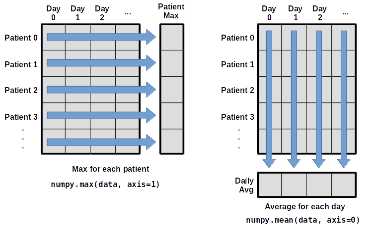
To find the maximum inflammation reported for each patient, you would apply the max function moving across the columns (axis 1). To find the daily average inflammation reported across patients, you would apply the mean function moving down the rows (axis 0).

To support this functionality, most array functions allow us to specify the axis we want to work on. If we ask for the max across axis 1 (columns in our 2D example), we get:

PYTHON

print(numpy.max(data, axis=1))

OUTPUT

[18. 18. 19. 17. 17. 18. 17. 20. 17. 18. 18. 18. 17. 16. 17. 18. 19. 19.
 17. 19. 19. 16. 17. 15. 17. 17. 18. 17. 20. 17. 16. 19. 15. 15. 19. 17.
 16. 17. 19. 16. 18. 19. 16. 19. 18. 16. 19. 15. 16. 18. 14. 20. 17. 15.
 17. 16. 17. 19. 18. 18.]

As a quick check, we can ask this array what its shape is. We expect 60 patient maximums:

PYTHON

print(numpy.max(data, axis=1).shape)

OUTPUT

(60,)

The expression (60,) tells us we have a one-dimensional array of 60 values. This data holds the maximum inflammation recorded for each patient.

If we ask for the average across/down axis 0 (rows in our 2D example), we get:

PYTHON

print(numpy.mean(data, axis=0))

OUTPUT

[ 0.          0.45        1.11666667  1.75        2.43333333  3.15
  3.8         3.88333333  5.23333333  5.51666667  5.95        5.9
  8.35        7.73333333  8.36666667  9.5         9.58333333 10.63333333
 11.56666667 12.35       13.25       11.96666667 11.03333333 10.16666667
 10.          8.66666667  9.15        7.25        7.33333333  6.58333333
  6.06666667  5.95        5.11666667  3.6         3.3         3.56666667
  2.48333333  1.5         1.13333333  0.56666667]

Check the array shape. We expect 40 averages, one for each day of the study:

PYTHON

print(numpy.mean(data, axis=0).shape)

OUTPUT

(40,)

Similarly, we can apply the mean function to axis 1 to get the patients’ average inflammation over the duration of the study (60 values).

PYTHON

print(numpy.mean(data, axis=1))

OUTPUT

[5.45  5.425 6.1   5.9   5.55  6.225 5.975 6.65  6.625 6.525 6.775 5.8
 6.225 5.75  5.225 6.3   6.55  5.7   5.85  6.55  5.775 5.825 6.175 6.1
 5.8   6.425 6.05  6.025 6.175 6.55  6.175 6.35  6.725 6.125 7.075 5.725
 5.925 6.15  6.075 5.75  5.975 5.725 6.3   5.9   6.75  5.925 7.225 6.15
 5.95  6.275 5.7   6.1   6.825 5.975 6.725 5.7   6.25  6.4   7.05  5.9  ]

Challenge

Slicing Strings

A section of an array is called a slice. We can take slices of character strings as well:

PYTHON

element = 'oxygen'
print('first three characters:', element[0:3])
print('last three characters:', element[3:6])

OUTPUT

first three characters: oxy
last three characters: gen

What is the value of element[:4]? What about element[4:]? Or element[:]?

Show me the solution

OUTPUT

oxyg
en
oxygen

Challenge

Slicing Strings (continued)

What is element[-1]? What is element[-2]?

Show me the solution

OUTPUT

n
e

Challenge

Slicing Strings (continued)

Given those answers, explain what element[1:-1] does.

Show me the solution

Creates a substring from index 1 up to (not including) the final index, effectively removing the first and last letters from ‘oxygen’

Challenge

Slicing Strings (continued)

How can we rewrite the slice for getting the last three characters of element, so that it works even if we assign a different string to element? Test your solution with the following strings: carpentry, clone, hi.

Show me the solution

PYTHON

element = 'oxygen'
print('last three characters:', element[-3:])
element = 'carpentry'
print('last three characters:', element[-3:])
element = 'clone'
print('last three characters:', element[-3:])
element = 'hi'
print('last three characters:', element[-3:])

OUTPUT

last three characters: gen
last three characters: try
last three characters: one
last three characters: hi

Pandas

---

Pandas is a Python library for data manipulation and analysis, providing powerful data structures like DataFrame and Series along with a wide range of functions for tasks such as data cleaning, preparation, and exploration. It is widely used in data science and machine learning workflows for its ease of use and flexibility.

We will now use the Iris dataset as an example of a dataset that does not just consist of numbers. This allows us to demonstrate some of the strengths of the Pandas library for inspecting structure and contents. To read in the dataset:

PYTHON

import pandas as pd

PYTHON

iris_df = pd.read_csv("../iris.csv")

Inspecting a Dataset

To understand the structure of the Iris dataset, we can use various methods provided by Pandas:

PYTHON

print(iris_df.head())

PYTHON

print(iris_df.info())

PYTHON

print(iris_df.describe())

Understanding the contents and data types of a dataset is important for accurate analysis.

Manipulating DataFrames

Pandas provides powerful functionalities to manipulate DataFrames. Here are some examples:

Adding and Removing Columns

Adding:

PYTHON

iris_df['sepal.ratio'] = iris_df['sepal.length'] / iris_df['sepal.width']

Removing:

PYTHON

iris_df.drop('variety', axis=1, inplace=True)

Adding and removing rows

Adding:

PYTHON

new_row = {'sepal.length': 5.1, 'sepal.width': 3.5, 'petal.length': 1.4, 'petal.width': 0.2,}
iris_df.loc[len(iris_df)] = new_row

Removing:

PYTHON

iris_df.drop(0, inplace=True)
iris_df.reset_index(drop=True, inplace=True)

Subsetting Data

Subsetting allows us to select specific rows or columns based on conditions:

PYTHON

iris_df = pd.read_csv("data/iris.csv") # reset the dataset
# Select rows where 'petal.length' is greater than 5
subset_df = iris_df[iris_df['petal.length'] > 5]

PYTHON

# Select rows where 'variety' is 'Setosa' and 'petal.length' is less than 1.5
subset_df = iris_df[(iris_df['variety'] == 'Setosa') & (iris_df['petal.length'] < 1.5)]

Key Points

• Remember array indices start at 0, not 1.
• Remember low:high to specify a slice that includes the indices from low to high-1.
• It’s good practice, especially when you are starting out, to use comments such as # explanation to explain what you are doing.
• We have shown some simple examples but you could slice your data in much more complicated ways depending on your requirements.
• It is hard to get an understanding of the data by just reading the raw numbers.