Visualising Tabular Data

Overview

Questions

• How can I visualise tabular data in Python?
• How can I generate several plots together?

Objectives

• Plot simple graphs from data.
• Plot multiple graphs in a single figure.

Visualizing data

---

The mathematician Richard Hamming once said, “The purpose of computing is insight, not numbers,” and the best way to develop insight is often to visualise data. Visualisation could take an entire course of its own, but for now we can explore a few features of Python’s matplotlib library here. While there is no official plotting library, matplotlib is the de facto standard. First, we will import the pyplot module from matplotlib and use two of its functions to create and display a heat map of our data:

Prerequisite

Episode Prerequisites

If you are continuing in the same notebook from the previous episode, you already have a data variable and have imported numpy. If you are starting a new notebook at this point, you need the following two lines:

PYTHON

import numpy as np
data = np.loadtxt(fname='../data/inflammation-01.csv', delimiter=',')

PYTHON

# you may need to %pip install matplotlib
import matplotlib.pyplot as plt
image = plt.imshow(data)
cbar = plt.colorbar()
plt.show()

Each row in the heat map corresponds to a patient in the clinical trial dataset, and each column corresponds to a day in the dataset. Blue pixels in this heat map represent low values, while yellow pixels represent high values. As we can see, the general number of inflammation flare-ups for the patients rises and falls over a 40-day period.

So far so good as this is in line with our knowledge of the clinical trial and Dr. Maverick’s claims:

• the patients take their medication once their inflammation flare-ups begin
• it takes around 3 weeks for the medication to take effect and begin reducing flare-ups
• and flare-ups appear to drop to zero by the end of the clinical trial.

Now let’s take a look at the average inflammation over time:

PYTHON

ave_inflammation = numpy.mean(data, axis=0)
ave_plot = plt.plot(ave_inflammation)
plt.show()

Here, we have put the average inflammation per day across all patients in the variable ave_inflammation, then asked matplotlib.pyplot to create and display a line graph of those values. The result is a reasonably linear rise and fall, in line with Dr. Maverick’s claim that the medication takes 3 weeks to take effect. But a good data scientist doesn’t just consider the average of a dataset, so let’s have a look at two other statistics:

PYTHON

max_plot = plt.plot(numpy.amax(data, axis=0))
plt.show()

PYTHON

min_plot = plt.plot(numpy.amin(data, axis=0))
plt.show()

The maximum value rises and falls linearly, while the minimum seems to be a step function. Neither trend seems particularly likely, so it’s likely there is something wrong with Dr Maverick’s data. This insight would have been difficult to reach by examining the numbers themselves without visualisation tools.

Grouping plots

You can group similar plots in a single figure using subplots. The script below uses a number of new commands. The function matplotlib.pyplot.figure() creates a figure into which we will place all of our plots. The parameter figsize tells Python how big to make this space. Each subplot is placed into the figure using its add_subplot method. The add_subplot method takes three parameters. The first denotes how many total rows of subplots there are, the second parameter refers to the total number of subplot columns, and the final parameter denotes which subplot your variable is referencing (left-to-right, top-to-bottom). Each subplot is stored in a different variable (axes1, axes2, axes3). Once a subplot is created, the axes can be titled using the set_xlabel() command (or set_ylabel()). Here are our three plots side by side:

PYTHON

data = numpy.loadtxt(fname='../data/inflammation-01.csv', delimiter=',')

fig = plt.figure(figsize=(10.0, 3.0))

axes1 = fig.add_subplot(1, 3, 1)
axes2 = fig.add_subplot(1, 3, 2)
axes3 = fig.add_subplot(1, 3, 3)

axes1.set_ylabel('average')
axes1.plot(numpy.mean(data, axis=0))

axes2.set_ylabel('max')
axes2.plot(numpy.amax(data, axis=0))

axes3.set_ylabel('min')
axes3.plot(numpy.amin(data, axis=0))

fig.tight_layout()

plt.savefig('inflammation.png')
plt.show()

The call to loadtxt reads our data, and the rest of the program tells the plotting library how large we want the figure to be, that we’re creating three subplots, what to draw for each one, and that we want a tight layout. (If we leave out that call to fig.tight_layout(), the graphs will actually be squeezed together more closely.)

The call to savefig stores the figure as a graphics file. This can be a convenient way to store your plots for use in other documents, web pages etc. The graphics format is automatically determined by Matplotlib from the file name ending we specify; here PNG from ‘inflammation.png’. Matplotlib supports many different graphics formats, including SVG, PDF, and JPEG.

Matplotlib cheatsheet 1 Matplotlib cheatsheet 2

Key Points

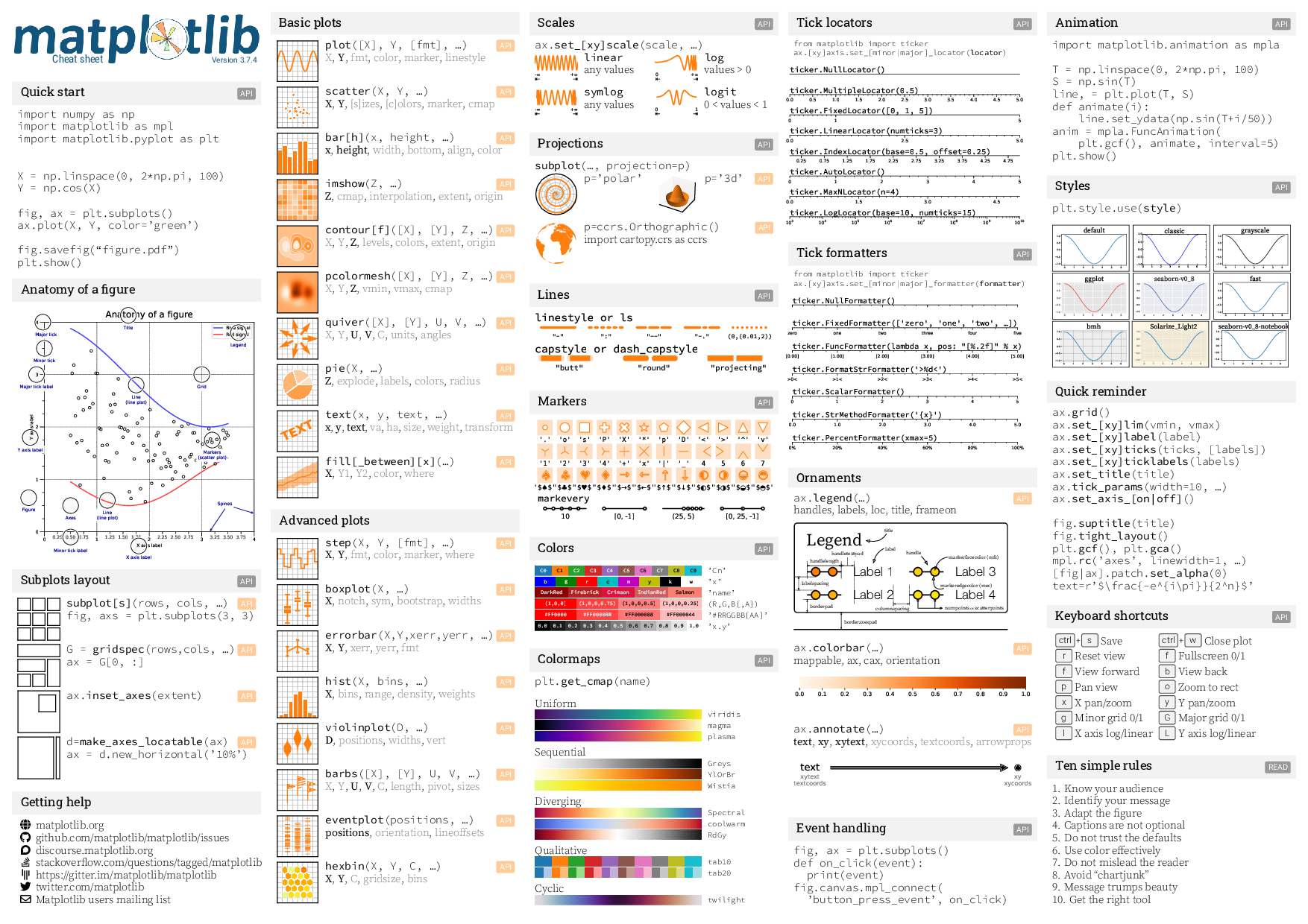
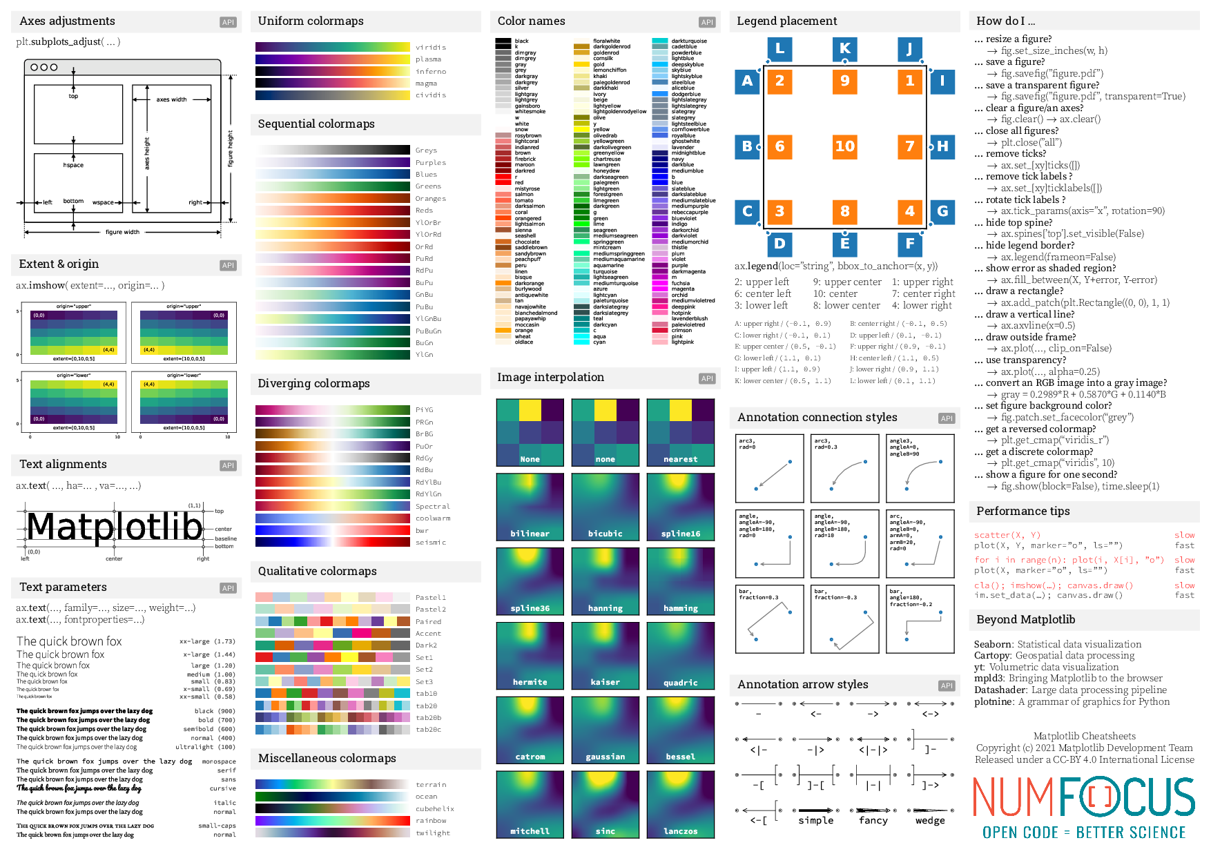
• We can easily visualise data using matplotlib.
• There are other libraries that are popular (e.g., seaborn).
• Getting figures “paper ready” can take a bit of time and effort.